Directional Flow
Tiling Liquid
- Align a texture with the flow direction.
- Partition the surface into tiles.
- Seamlessly blend tiles.
- Obfuscate visual artifacts.
This is the second tutorial in a series about creating the appearance of flowing materials. It comes after Texture Distortion and is about aligning patterns with the flow, instead of distorting them.
This tutorial is made with Unity 2017.4.4f1.
Anisotropic Patterns
When distorting a texture to simulate flow, it can end up getting stretched or squashed in any direction. This means that it must look good no matter how it gets deformed. This is only possible with isotropic patterns. Isotropic means that the image appears similar in all directions. This is the case for the water texture that we used in the previous tutorial.
Rippling Water
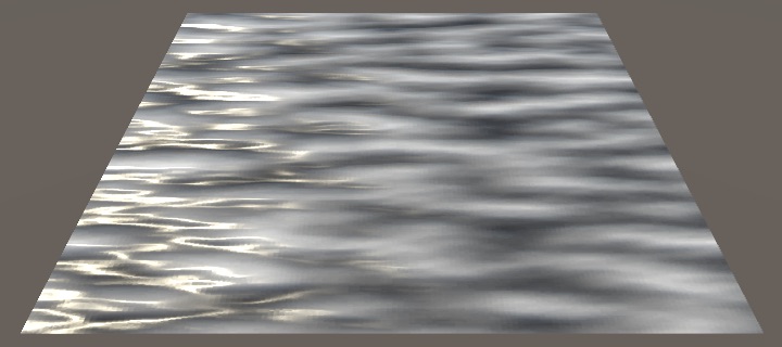
While the illusion of flow can be convincing, the patterns created by distorting an isotropic pattern do not look like real water. This is most obvious when observing a still image of the effect, instead of an animation. You can't really tell what the flow direction is supposed to be. That's because the alignment of the waves and ripples is wrong. They're elongated along the flow direction, instead of being perpendicular to it.

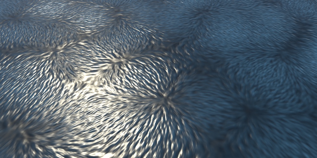
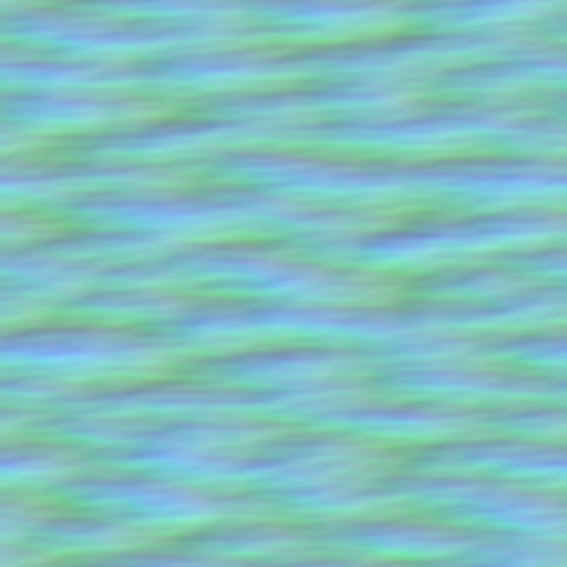
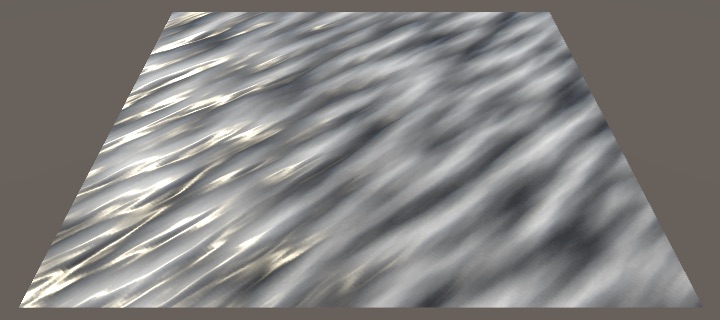
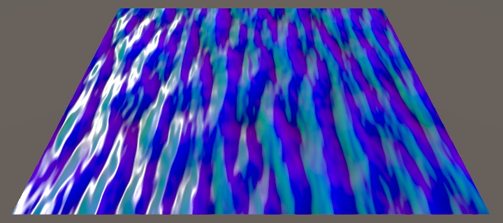
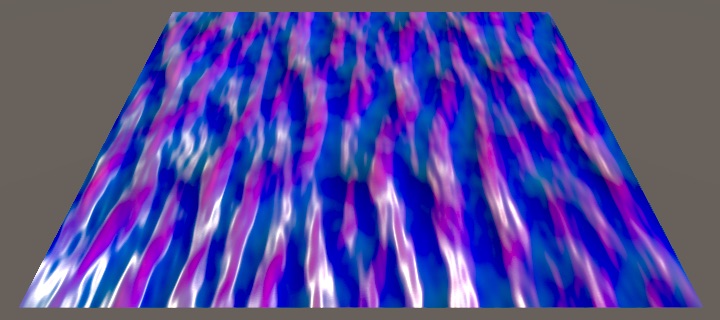
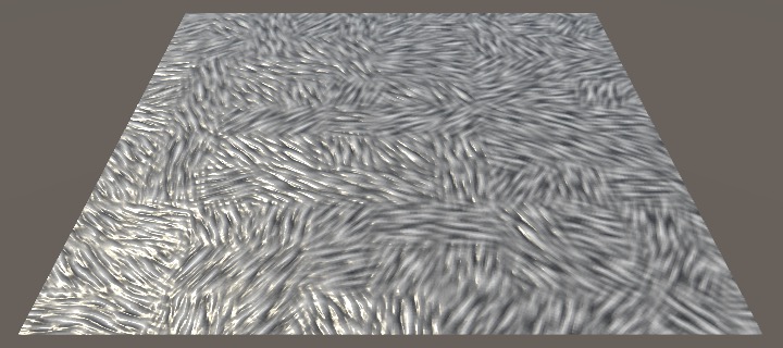
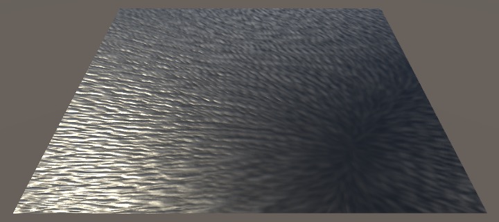
The distortion effect works best for either very turbulent or very sluggish flows. It doesn't work well for more calm flows that manifest clear ripple patterns, because such ripples have a clear direction to them. They're anisotropic. Here is an alternative water texture containing such ripples. It's made the same way as the other texture, but with a different pattern, and the derivatives are scaled by a factor of 0.025 relative to the height data.
Import the texture, make sure that it's not in sRGB mode, and use it for the pattern of the distortion effect.
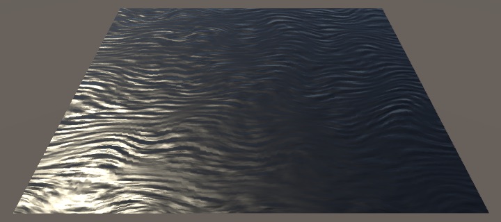
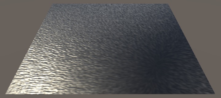
There is now a clear visual direction, even when there is no animation. However, the pattern isn't aligned with the flow, so the implied direction is incorrect. We have to use a different approach if we want to visualize proper ripples.
Directional Flow Shader
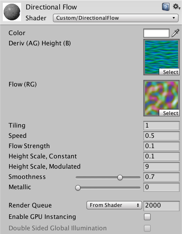
In this tutorial we'll create a different flow shader. Instead of distorting a texture, it will align it with the flow. Duplicate the DistortionFlow shader and rename it to DirectionalFlow. We'll leave all parameters the same, except that we won't use the jump parameters, so remove those. Also, we won't bother with an albedo texture, so the derivative-height data can be supplied via the main texture. And we won't need noise to offset a phase blend, so we're only interested in the RG channels of the flow map.
We'll start by reducing the surf function to just sampling the derivative-height data, using the squared height for albedo and setting the normal vector.
Shader "Custom/DirectionalFlow" {
Properties {
_Color ("Color", Color) = (1,1,1,1)
[NoScaleOffset] _MainTex ("Deriv (AG) Height (B)", 2D) = "black" {}
[NoScaleOffset] _FlowMap ("Flow (RG)", 2D) = "black" {}
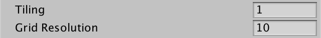
_Tiling ("Tiling", Float) = 1
_Speed ("Speed", Float) = 1
_FlowStrength ("Flow Strength", Float) = 1
_HeightScale ("Height Scale, Constant", Float) = 0.25
_HeightScaleModulated ("Height Scale, Modulated", Float) = 0.75
_Glossiness ("Smoothness", Range(0,1)) = 0.5
_Metallic ("Metallic", Range(0,1)) = 0.0
}
SubShader {
Tags { "RenderType"="Opaque" }
LOD 200
CGPROGRAM
#pragma surface surf Standard fullforwardshadows
#pragma target 3.0
#include "Flow.cginc"
sampler2D _MainTex, _FlowMap;
float _Tiling, _Speed, _FlowStrength;
float _HeightScale, _HeightScaleModulated;
struct Input {
float2 uv_MainTex;
};
half _Glossiness;
half _Metallic;
fixed4 _Color;
float3 UnpackDerivativeHeight (float4 textureData) {
float3 dh = textureData.agb;
dh.xy = dh.xy * 2 - 1;
return dh;
}
void surf (Input IN, inout SurfaceOutputStandard o) {
float2 uv = IN.uv_MainTex * _Tiling;
float3 dh = UnpackDerivativeHeight(tex2D(_MainTex, uv));
fixed4 c = dh.z * dh.z * _Color;
o.Albedo = c.rgb;
o.Normal = normalize(float3(-dh.xy, 1));
o.Metallic = _Metallic;
o.Smoothness = _Glossiness;
o.Alpha = c.a;
}
ENDCG
}
FallBack "Diffuse"
}
Create a material with this shader, using the same settings as the distortion material, except now using the ripple pattern and with tiling set to 1. When applied to the quad, we end up with simply the ripple pattern. The pattern is aligned to correspond with a flow along the V axis. The default is that it flows up, but as the pattern is symmetrical in works in the opposite direction too.
Aligning With the Flow
Now that we have an anisotropic pattern, we need to find a way to align it with a flow direction. We'll first try this with a fixed and controlled direction, and once that's working move on to using the flow map.
UV for Directional Flow
Aligning a texture with a direction is a matter of transforming UV coordinates. This is a fundamental operation useful for flow simulation, so we'll add a function for that to our Flow include file. Name it DirectionalFlowUV. It needs the original UV coordinates and a flow vector as parameters. Also give it tiling and time parameters, similar to the FlowUVW function. As it won't perform deformation that requires a time reset, no phase data nor a time-blending weight are involved.
float2 DirectionalFlowUV (
	float2 uv, float2 flowVector, float tiling, float time
) {}
We begin by simply scrolling up, moving the pattern in the positive V direction, by subtracting the time from the V coordinate. Then apply the tiling.
float2 DirectionalFlowUVW (
	float2 uv, float2 flowVector, float tiling, float time
) {
	uv.y -= time;
	return uv * tiling;
}
Use this function in our shader to get the final flow UV coordinates. We'll supply it with float(0, 1) as the flow vector—`[[0],[1]]` representing the default orientation—the tiling property, and the time modulated by the speed. Then we use the result to sample the pattern.
		void surf (Input IN, inout SurfaceOutputStandard o) {
			//float2 uv = IN.uv_MainTex * _Tiling;
			float time = _Time.y * _Speed;
			float2 uvFlow = DirectionalFlowUV(
				IN.uv_MainTex, float2(0, 1), _Tiling, time
			);
			float3 dh = UnpackDerivativeHeight(tex2D(_MainTex, uvFlow));
			…
		}
The result is the same as before, but with movement.
Texture Rotation
To rotate UV coordinates, we need a 2D rotation matrix, as described in the Rendering 1, Matrices tutorial. If the flow vector `[[x],[y]]` is of unit length, then it represents a point on the unit circle. As `[[0],[1]]` corresponds to no rotation, the X coordinate represents the sine of some rotation angle `theta` (theta), while the Y coordinate represents the cosine of the same angle. Also, the flow vector `[[1],[0]]` represents flow in the U direction, to the right. So the flow vector can be interpreted as `[[sin theta],[cos theta]]` for a clockwise rotation.
The Rendering 1, Matrices tutorial defined a 2D rotation matrix as `[[cos theta,-sin theta],[sin theta,cos theta]]`, but that represents a counterclockwise rotation. As we need a clockwise rotation, we have to flip the sign of `sin theta`, which gives us the final rotation matrix `[[y,x],[-x,y]]`.
Because our flow map doesn't contain vectors of unit length, we have to normalize them first. Then construct the matrix using that direction vector, via the float2x2 construction function. Multiply that matrix with the original UV coordinates, using the mul function. After that's done the time offset and tiling should be applied.
float2 DirectionalFlowUV (
	float2 uv, float2 flowVector, float tiling, float time
) {
	float2 dir = normalize(flowVector.xy);
	uv = mul(float2x2(dir.y, dir.x, -dir.x, dir.y), uv);
	uv.y -= time;
	return uv * tiling;
}
Let's test whether this works, by using the flow vector `[[1],[1]]`. That should result in a pattern that's rotated 45° clockwise.
			float2 uvFlow = DirectionalFlowUV(
				IN.uv_MainTex, float2(1, 1), _Tiling, time
			);
We get a counterclockwise rotation instead. That's because we're not rotating the pattern itself, but the UV coordinates. To get the correct result, we have to rotate them in the opposite direction, just like we have to subtract the time to scroll in a positive direction. So we have to use the counterclockwise rotation matrix after all.
uv = mul(float2x2(dir.y, -dir.x, dir.x, dir.y), uv);
To make sure that all flow vectors are now converted to correct rotations, let's rotate based on time, using `[[sin time],[cos time]]`. Set the material's speed to zero so the only movement is causes by the rotation, otherwise it's hard to interpret the movement.
			float uvFlow = DirectionalFlowUV(
				IN.uv_MainTex, float2(sin(_Time.y), cos(_Time.y)), _Tiling, time
			);
The rotation works as it should. The animation also reveals that the rotation is centered on the bottom left of the quad, which corresponds to the origin of the UV space. While we could offset the rotation so it is centered on another point, this isn't necessary.
Rotating Derivatives
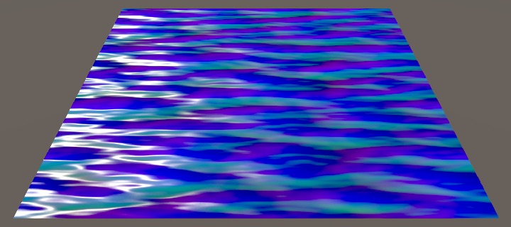
Although the pattern rotates correctly, there is something wrong with the normal vectors. This might not be immediately obvious, but it becomes glaring once you pay attention to how the surface should look. It's easiest to visualize by using the derivatives to colorize the material.
o.Albedo = dh; //c.rgb;
At zero rotation—due to the anisotropic pattern—we mostly see green, with little red. Blue can be ignored, because that's the height.
What colors do we see when the pattern is rotated 90°?
We still see the same colors. This would be correct if it was just color data. But these are derivatives, which represent surface curvature. When the surface rotates, so should its curvature, but that's not happening. This means that the lighting is affected by changes in position, but not rotation.
To keep the lighting correct, we have to rotate the normal vectors, which is the same as rotating the derivatives. As DirectionalFlowUV is responsible for the rotation, it makes sense that it also gives us the matrix to use for vector rotation. Let's make that possible by adding an output parameter to it. In this case, we do need the proper clockwise rotation matrix.
float2 DirectionalFlowUV (
	float2 uv, float2 flowVector, float tiling, float time,
	out float2x2 rotation
) {
	float2 dir = normalize(flowVector.xy);
	rotation = float2x2(dir.y, dir.x, -dir.x, dir.y);
	uv = mul(float2x2(dir.y, -dir.x, dir.x, dir.y), uv);
	uv.y -= time;
	return uv * tiling;
}
Supply a variable for this new output, then use it to rotate the derivatives that we sample later, with another matrix multiplication.
			float time = _Time.y * _Speed;
			float2x2 derivRotation;
			float2 uvFlow = DirectionalFlowUV(
				IN.uv_MainTex, float2(sin(_Time.y), cos(_Time.y)), _Tiling, time,
				derivRotation
			);
			float3 dh = UnpackDerivativeHeight(tex2D(_MainTex, uvFlow));
			dh.xy = mul(derivRotation, dh.xy);
Now that the derivatives rotate as well, the colors change too. At 90° rotation, red and green have swapped. Now we can restore the original color.
o.Albedo = c.rgb;
Sampling the Flow
The next step is to use the flow map to control the rotation. Sample the map and supply its data to DirectionalFlowUV.
			float2 flow = tex2D(_FlowMap, IN.uv_MainTex).rg;
			flow = flow.xy * 2 - 1;
			float2 uvFlow = DirectionalFlowUV(
				IN.uv_MainTex, flow, _Tiling, time,
				derivRotation
			);
But because we normalize the flow vectors, we lose the speed information. Fortunately, we stored the speed in the flow map's B channel, so we can pass that to DirectionalFlowUV as well. Adjust and rename its parameter for that, then modulate the time with the speed before adding it.
float2 DirectionalFlowUV (
	float2 uv, float3 flowVectorAndSpeed, float tiling, float time,
	out float2x2 rotation
) {
	float2 dir = normalize(flowVectorAndSpeed.xy);
	rotation = float2x2(dir.y, dir.x, -dir.x, dir.y);
	uv = mul(float2x2(dir.y, -dir.x, dir.x, dir.y), uv);
	uv.y -= time * flowVectorAndSpeed.z;
	return uv * tiling;
}
Retrieve the speed data and pass it to the function. But before that, let's also modulate it with the Flow Strength shader property. The distortion shader uses this property to control the amount of distortion, but it also affects the animation speed. While we don't really need to do this in the directional shader, it makes it easier to configure the exact same speed for both shaders. That is convenient when comparing the effects.
			float3 flow = tex2D(_FlowMap, IN.uv_MainTex).rgb;
			flow.xy = flow.xy * 2 - 1;
			flow.z *= _FlowStrength;
			float2 uvFlow = DirectionalFlowUV(
				IN.uv_MainTex, flow, _Tiling, time,
				derivRotation
			);
Unfortunately—like with the distortion shader—we get a heavily distorted an unusable result. Rotating each fragment independently rips the pattern apart. This wasn't a problem when we used a uniform direction. We'll have to come up with a solution.
Tiled Flow
The distortion approach had a temporal problem, because we were forced to reset the distortion at some point, to keep the pattern intact. We hid that by blending between two different phases across time. The directional approach has this problem too, but it's of a different nature. While the pattern breaks up more as time progresses, it's already destroyed at time zero, without any animation. So resetting time won't help.
Instead, there is a discontinuity where there is a difference in orientation. This is a spatial problem, not a temporal one. The solution is once again to hide the problem by blending. But now we have to blend in space, not time. And we're dealing with a 2D surface, not with 1D time, so it will be more complex.
What we'll do is try to find a compromise between the perfect result of a uniform flow and the desired result of using a different flow direction per fragment. That compromise is to divide the surface into regions. We'll simply use a grid of square tiles. Each tile has a uniform flow, so won't suffer from any distortion. Then we'll blend each tile with its neighbors, to hide the discontinuities between them. This approach was first publicly described by Frans van Hoesel in 2010, as the Tiled Directional Flow algorithm. We'll create a variant of it.
Flow Grid
To split the surface into tiles, we need to decide on a grid resolution. We'll make that configurable via a shader property, using a default of 10.
		_Tiling ("Tiling", Float) = 1
		_GridResolution ("Grid Resolution", Float) = 10
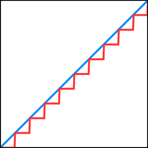
Cutting the flow map into tiles can be done by multiplying the UV used for sampling the map by the grid resolution, then discarding the fractional part. That gives us tiles with fixed UV coordinates, from 0 up to the grid resolution. To convert that back to a range from 0 to 1, divide by the tiled coordinates by the grid resolution.
		float _Tiling, _GridResolution, _Speed, _FlowStrength;
		float _HeightScale, _HeightScaleModulated;

		…

		void surf (Input IN, inout SurfaceOutputStandard o) {
			float time = _Time.y * _Speed;
			float2x2 derivRotation;
			float2 uvTiled =
				floor(IN.uv_MainTex * _GridResolution) / _GridResolution;
			float3 flow = tex2D(_FlowMap, uvTiled).rgb;
			…
		}
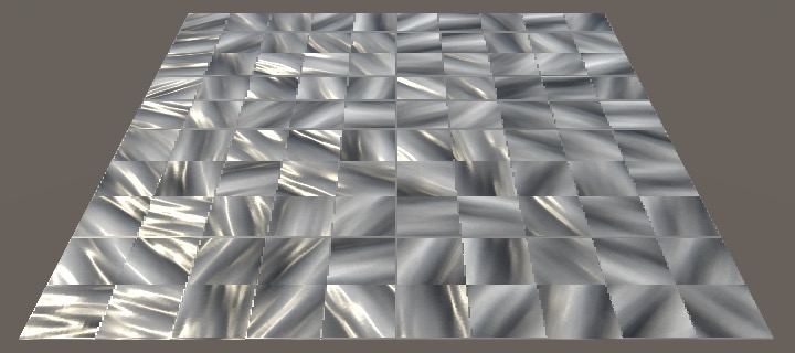
Blending Cells
At this point we have clearly distinguishable grid cells, each containing an undistorted pattern. The next step is to blend them. This requires us to sample multiple cells per fragment. So let's move the code to compute the derivative plus height data to a new FlowCell function. Initally, all it needs are the original UV coordinates and the scaled time.
		float3 FlowCell (float2 uv, float time) {
		    float2x2 derivRotation;
			float2 uvTiled =
				floor(uv * _GridResolution) / _GridResolution;
			float3 flow = tex2D(_FlowMap, uvTiled).rgb;
			flow.xy = flow.xy * 2 - 1;
			flow.z *= _FlowStrength;
			float2 uvFlow = DirectionalFlowUV(
				uv, flow, _Tiling, time,
				derivRotation
			);
			float3 dh = UnpackDerivativeHeight(tex2D(_MainTex, uvFlow));
			dh.xy = mul(derivRotation, dh.xy);
			return dh;
		}

		void surf (Input IN, inout SurfaceOutputStandard o) {
			float time = _Time.y * _Speed;
			//float2x2 derivRotation;
			//…
			//dh.xy = mul(derivRotation, dh.xy);
			float2 uv = IN.uv_MainTex;
			float3 dh = FlowCell(uv, time);
			fixed4 c = dh.z * dh.z * _Color;
			…
		}
Sampling a different cell can be done by adding an offset before flooring the UV coordinates to find the fixed flow. Add a parameter for that to FlowCell.
		float3 FlowCell (float2 uv, float2 offset, float time) {
		    float2x2 derivRotation;
			float2 uvTiled =
				floor(uv * _GridResolution + offset) / _GridResolution;
			…
		}
Let's first try an offset of one unit in the U dimension. That means that we end up sampling one cell to the right, visually shifting the flow data one step to the left.
float3 dh = FlowCell(uv, float2(1, 0), time);
To blend the cells horizontally, we have to sample both the original and the offset cell per tile. We'll designate the original data as A and the offset data as B. First, let's just average them, giving each a weight of 0.5 and summing that.
			float3 dhA = FlowCell(uv, float2(0, 0), time);
			float3 dhB = FlowCell(uv, float2(1, 0), time);
			float3 dh = dhA * 0.5 + dhB * 0.5;
Each tile now contains the same amount of A and B everywhere. Next, we have to transition from A to B along the U dimension. We can do this by linearly interpolating between A and B. The fractional part of the scaled U coordinate is the value `t` that we can use to interpolate the weights. Let's visualize it, by using it as the albedo.
			float3 dhA = FlowCell(uv, float2(0, 0), time);
			float3 dhB = FlowCell(uv, float2(1, 0), time);

			float t = frac(uv.x * _GridResolution);

			float3 dh = dhA * 0.5 + dhB * 0.5;
			fixed4 c = dh.z * dh.z * _Color;
			o.Albedo = t; // c.rgb;
The A cell starts at full strength on the left side of each tile, where `t` is zero. And it should be gone when `t` reaches 1 on the right side. So the weight of A is `t-1`. B is the other way around, so its weight is simply `t`.
			float3 dhA = FlowCell(uv, float2(0, 0), time);
			float3 dhB = FlowCell(uv, float2(1, 0), time);

			float t = frac(uv.x * _GridResolution);
			float wA = 1 - t;
			float wB = t;

			float3 dh = dhA * wA + dhB * wB;
			fixed4 c = dh.z * dh.z * _Color;
			o.Albedo = c.rgb;
Overlapping Cells
Although interpolation between the cells should eliminate the horizontal discontinuity, we can still see lines that make the grid obvious. These lines are artifacts caused by the sudden jump of the UV coordinates used to sample the flow map. The suddenly large UV delta triggers the GPU to select a different mipmap level along the grid line, corrupting the flow data. While we could eliminate these artifacts by eliminating mipmaps, this isn't desirable. It would be better if we could hide them some other way.
We can hide the lines by making sure that the cell weights are zero at their edges, which is where the artifact lines are. But the weight function `t` reset each tile, so we have sawtooth waves that are both 0 and 1 on the edge. Thus although one side is always fine, the other suffers from the artifacts.
To solve this problem, we have to overlap the cells. That way we can alternate between them and use one to hide the artifacts of the other. First, halve the offset of the second cell. It's most convenient to do this inside FlowCell, so we can keep using whole numbers for the offset argument. The shader compiler will get rid of the extra calculations away.
		float3 FlowCell (float2 uv, float2 offset, float time) {
		    offset *= 0.5;
			…
		}
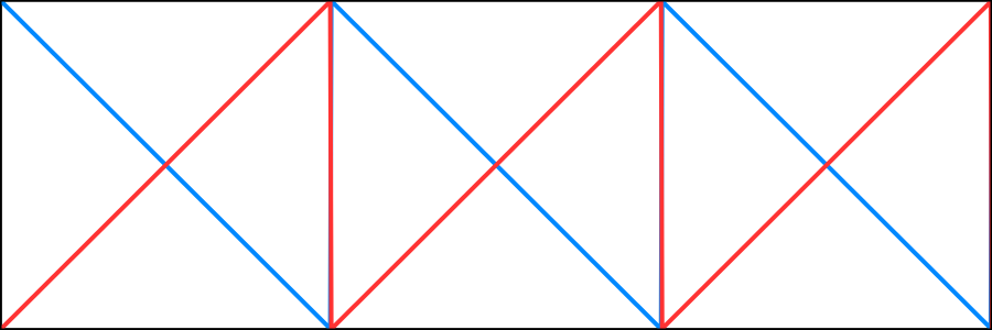
The horizontal cells are now overlapping, occurring at twice the frequency than the tiles that we actually use. Next, we have to correctly blend between the cells again. This is done by replacing `t` with `|2t-1|`, turning it into a triangle wave that is zero on both sides of a tile and 1 in the middle.

The result of this change is that the weight of A is now zero on both sides of each tile. It is at full strength halfway. And it's the other way around for B, which has zero weight in the middle of each tile. And because we offset B by only half a tile now, that's exactly where its artifact line would've shown up.
			float t = abs(2 * frac(uv.x * _GridResolution) - 1);
			float wA = 1 - t;
			float wB = t;
Now that we can blend without artifacts, let's also do this vertically. Add cells C and D, both offset by one step in the V dimension relative to A and B.
			float3 dhA = FlowCell(uv, float2(0, 0), time);
			float3 dhB = FlowCell(uv, float2(1, 0), time);
			float3 dhC = FlowCell(uv, float2(0, 1), time);
			float3 dhD = FlowCell(uv, float2(1, 1), time);

			float t = abs(2 * frac(uv.x * _GridResolution) - 1);
			float wA = 1 - t;
			float wB = t;
			float wC = 1 - t;
			float wD = t;

			float3 dh = dhA * wA + dhB * wB + dhC * wC + dhD * wD;
The weights of A and B must now be multiplied by `1-t` in the V dimension, and by `t` for C and D. Each dimension gets its own `t` value, which we can do by changing it to float2 and deriving it from both UV coordinates.
			float2 t = abs(2 * frac(uv * _GridResolution) - 1);
			float wA = (1 - t.x) * (1 - t.y);
			float wB = t.x * (1 - t.y);
			float wC = (1 - t.x) * t.y;
			float wD = t.x * t.y;

Sampling At Cell Centers
Currently, we're sampling the flow at the bottom left corner of each tile. But that doesn't line up with the way that we blend the cells. The result is a misaligned blend between flow data, which makes the grid more obvious than it should be. Instead, we should sample the flow at the center of each cell, where its weight is 1. In the case of cell A, that's in the middle of each tile, so its sample point needs to be shifted there. The same is true for B, at least in the V dimension. Because B is already offset by half a tile in the U dimension, it doesn't need a horizontal shift. And C and D are fine in the V dimension, but C needs a horizontal shift.
In general, we have to shift half a tile when there isn't an offset, and vice versa. We can conveniently do this in FlowCell by taking 1 minus the unscaled offset and halving that. Then add that to the UV coordinates after flooring, before the division.
		    float2 shift = 1 - offset;
		    shift *= 0.5;
		    offset *= 0.5;
			float2 uvTiled =
				(floor(uv * _GridResolution + offset) + shift) / _GridResolution;
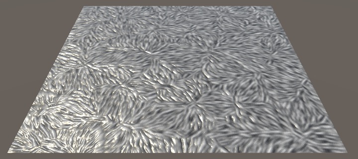
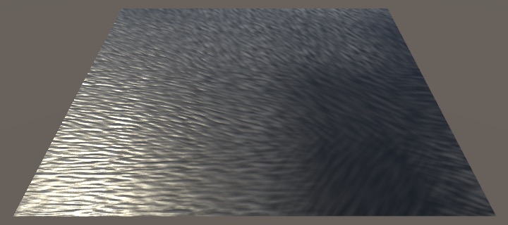
We're now correctly using the flow data, but how accurate we are depends on the grid resolution. The higher the resolution, the smoother the flow curves. But we cannot make the resolution too high, because that doesn't allow room for the ripple pattern to show up.
Increasing the tiling allows the resolution to go higher, but also makes the ripples smaller. You have to find a balance that works best for each situation. For example, a tiling of 5 combined with a grid resolution of 30 works well for the images in this tutorial. That makes it possible to see the flow, without the ripples becoming to small to see.
Scaling the Waves
Like we did for the distortion effect, let's also scale the strength of the derivative and height data, both using a constant factor and modulated by the flow strength.
		float3 FlowCell (float2 uv, float2 offset, float time) {
		    …
			dh.xy = mul(derivRotation, dh.xy);
			dh *= flow.z * _HeightScaleModulated + _HeightScale;
			return dh;
		}
Because of our spatial approach, it is now also possible to scale the pattern size based on the flow speed as well. Rapidly flowing streams have many small ripples, while slower regions have fewer larger ripples. We can support this by factoring the flow speed into the tiling.
			flow.z *= _FlowStrength;
			float tiling = flow.z * _Tiling;
			float2 uvFlow = DirectionalFlowUV(
				uv, flow, tiling, time,
				derivRotation
			);
This degenerates when the flow speed is very low—which is the case because we use a flow strength of 0.1—because the pattern becomes far too large. Only a very small region of the ripple pattern fits in each cell.
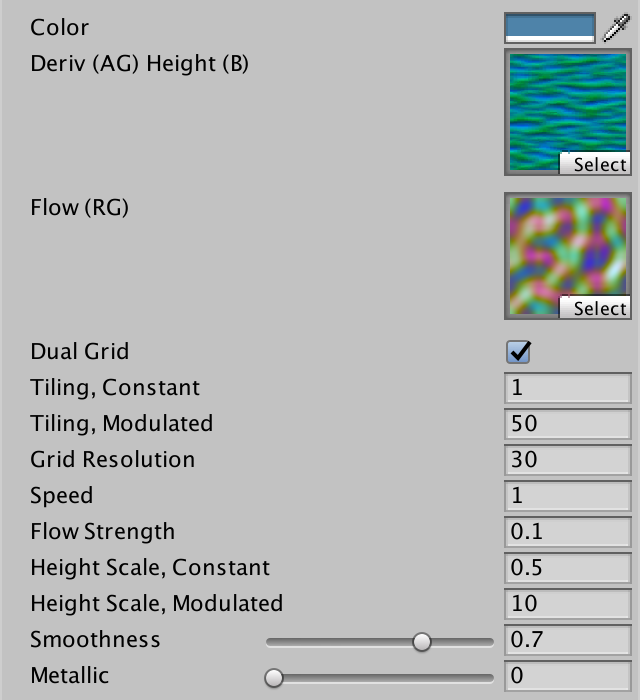
We can still scale the pattern, just in moderation. We can do this the same way that we scale the height, by making a property both for constant and modulated tiling. I'll set the constant tiling to 3 and the modulated tiling to 50. The modulate tiling has be to so high to compensate for the low flow speed.
		_Tiling ("Tiling, Constant", Float) = 1
		_TilingModulated ("Tiling, Modulated", Float) = 1
The final tiling becomes equal to the flow speed multiplied with the modulated tiling, plus the original constant tiling.
		float _Tiling, _TilingModulated, _GridResolution, _Speed, _FlowStrength;
		float _HeightScale, _HeightScaleModulated;

		…

		float3 FlowCell (float2 uv, float2 offset, float time) {
		    …
			float tiling = flow.z * _TilingModulated + _Tiling;
			…
		}
Hiding Artifacts
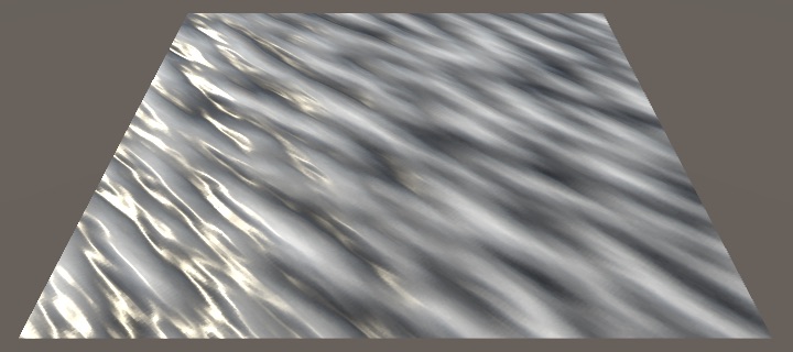
Although our directional flow shader is now functionally complete, there are unfortunately still some artifacts. While they're not always obvious, they still warrant attention.
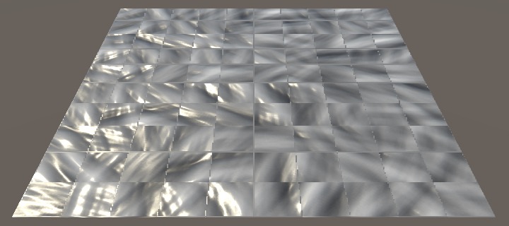
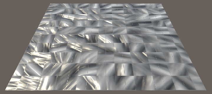
The most immediately obvious artifacts are visible tiling where the flow direction changes fairly quickly. This is quite pronounced for our flow map, because it has a lot of twists and turns. This can be solved by increasing the grid resolution, but will also require an increase of the tiling.
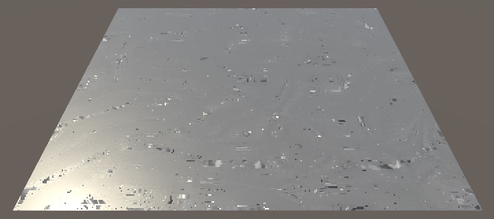
Nearly Uniform Flow
The really problematic artifacts appear in regions where there isn't much change in the flow. If the flow is truly uniform, then the tiling of the pattern cannot be hidden. To see this, force tiled UV coordinates to zero, so the same flow data is used everywhere.
float3 flow = tex2D(_FlowMap, uvTiled * 0).rgb;
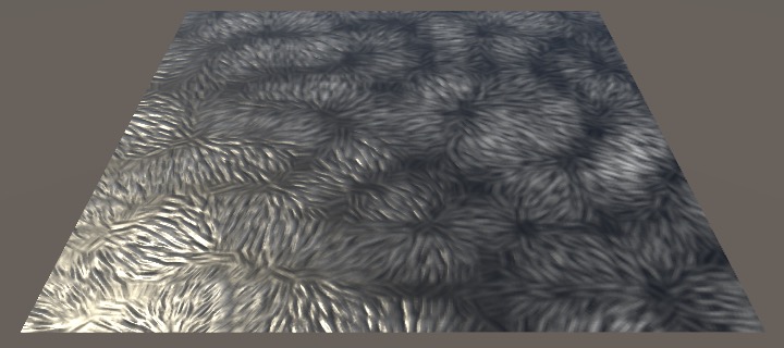
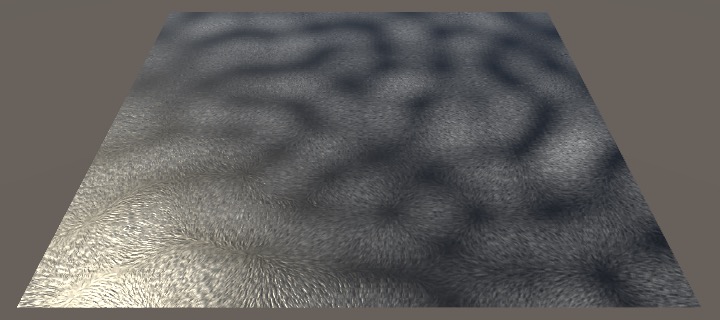
The visible tiling can be removed by simply using a larger ripple pattern, but that has its limits. The only way to truly prevent this is by ensuring there is at least some variety, maybe by adding noise when generating a flow map. This is a fine approach, because liquids rarely flow perfectly uniform. There are usually hidden or submerged factors that influence the flow in some way. So let's consider a mostly uniform flow, like a slowly curving current. We can see such a situation by temporarily scaling the flow sampling by 0.1.
float3 flow = tex2D(_FlowMap, uvTiled * 0.1).rgb;
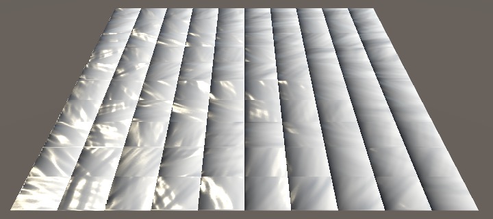
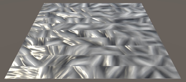
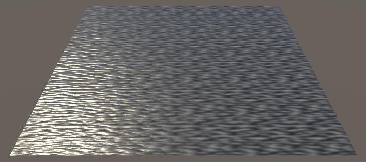
It is possible to spot pulsing patterns that match the flow during animation, but those are hard to notice with a quick glance. A more obvious manifestation of this problem shows up when setting the speed to zero. Suddenly, we can see streaks appear, caused by nearly the same region of the ripple pattern repeating with a slight offset, rotation, and scale.
Compression of the flow map and texture filtering can help mask these artifacts somewhat. When using an uncompressed flow map, the artifacts change and can become even more pronounced.
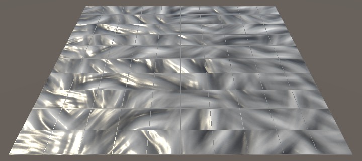
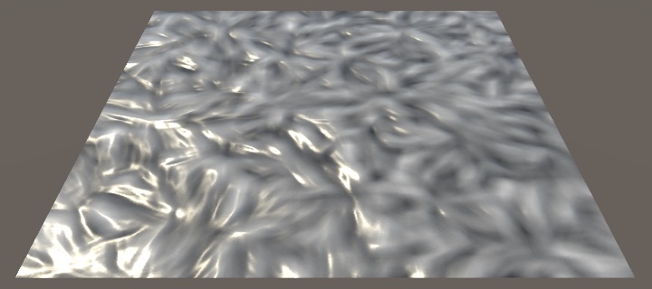
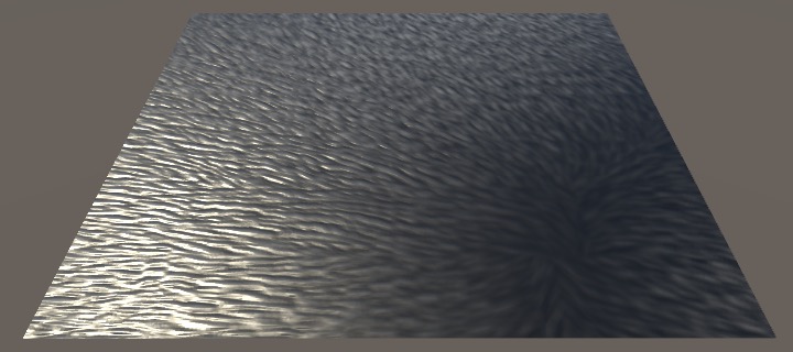
These problems are causes by quick pattern repetition. While decreasing the grid resolution helps to reduce this, it also makes the flow less smooth. Fortunately, we can obfuscate the repetition by jittering the UV coordinates when sampling the pattern per cell. Simply adding the cell offset suffices.
			float2 uvFlow = DirectionalFlowUV(
				uv + offset, flow, tiling, time,
				derivRotation
			);
As this increases the difference between cell patterns, it also adds more apparent animation. This makes the ripples more animated.
Spotting the Grid
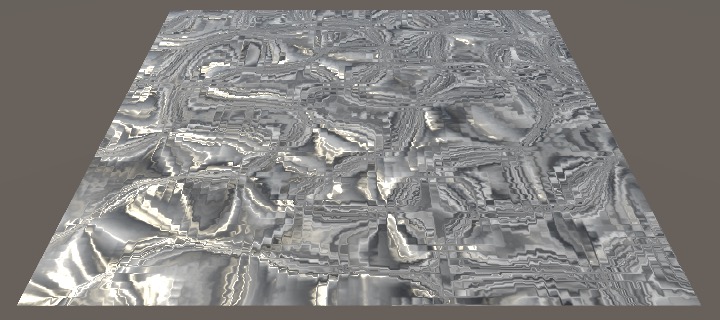
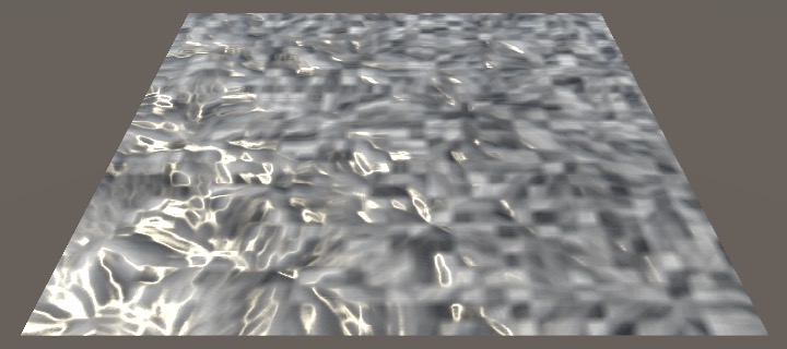
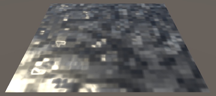
There is another kind of artifact, caused by blending between cells. If the difference in direction or speed is large enough, the tiling can become obvious. For example, set the grid resolution to 3 while we're still zoomed in on the flow map.
There are now clearly distinguishable tiles that are darker or lighter. This is caused by the different flow speeds per tile. But that's not the most problematic part. We can eliminate this by using a black color.
It is still possible to see the grid, when you pay attention to the specular reflections. That's because regions where cells are blended are flatter than those that are dominated by a single cell. As a result, specular reflections vary in a grid pattern. As this pattern is static, it stands out even more when the ripples are animated.
Mixing Grids
There is no easy way to get rid of the specular artifacts, like we couldn't completely eliminate the phase blend artifacts of the distortion effect, just obfuscate it with noise. In this case, perturbing the grid with noise won't make it less obvious. Also, smoothing the blend function won't eliminate them, in fact any change will make them more obvious.
The only way to eliminate the artifacts is to get rid of the transition between uniform and mixed regions, but that is impossible. The next best thing is to smudge the difference.
What we can do is sample the entire grid twice. If we offset the second grid by a quarter tile, then its sharpest regions correspond to the other grid's blurriest areas, and vice versa. If we then average those two grids, then we end up with a much more uniform blend.
Move the code that samples and combines the four cells to a new FlowGrid function.
		float3 FlowGrid (float2 uv, float time) {
		    float3 dhA = FlowCell(uv, float2(0, 0), time);
			float3 dhB = FlowCell(uv, float2(1, 0), time);
			float3 dhC = FlowCell(uv, float2(0, 1), time);
			float3 dhD = FlowCell(uv, float2(1, 1), time);

			float2 t = abs(2 * frac(uv * _GridResolution) - 1);
			float wA = (1 - t.x) * (1 - t.y);
			float wB = t.x * (1 - t.y);
			float wC = (1 - t.x) * t.y;
			float wD = t.x * t.y;

			return dhA * wA + dhB * wB + dhC * wC + dhD * wD;
		}

		void surf (Input IN, inout SurfaceOutputStandard o) {
			float time = _Time.y * _Speed;
			float2 uv = IN.uv_MainTex;
			//float3 dhA = FlowCell(uv, float2(0, 0), time);
			//…
			//float3 dh = dhA * wA + dhB * wB + dhC * wC + dhD * wD;
			float3 dh = FlowGrid(uv, time);
			fixed4 c = dh.z * dh.z * _Color;
			…
		}
We're now going to sample two grids, just like we sampled two phases for the distortion effect. Again, we can use a boolean parameter to indicate whether we want variant A or variant B. Then sample both and average them.
		float3 FlowGrid (float2 uv, float time, bool gridB) {
		    …
		}

		void surf (Input IN, inout SurfaceOutputStandard o) {
			…
			float3 dh = FlowGrid(uv, time, false);
			dh = (dh + FlowGrid(uv, time, true)) * 0.5;
			…
		}
In case of variant B, we have to shift the weight function. Add a quarter after scaling, before taking the fractional part.
			float2 t = uv * _GridResolution;
			if (gridB) {
			    t += 0.25;
			}
			t = abs(2 * frac(t) - 1);
We also have to tell FlowCell which variant we need. The alternative grid has to be offset by a quarter, and the sample shift has to be offset in the other direction to compensate.
		float3 FlowCell (float2 uv, float2 offset, float time, float gridB) {
		    float2 shift = 1 - offset;
		    shift *= 0.5;
		    offset *= 0.5;
		    if (gridB) {
		        offset += 0.25;
		        shift -= 0.25;
		    }
			…
		}

		float3 FlowGrid (float2 uv, float time, bool gridB) {
		    float3 dhA = FlowCell(uv, float2(0, 0), time, gridB);
			float3 dhB = FlowCell(uv, float2(1, 0), time, gridB);
			float3 dhC = FlowCell(uv, float2(0, 1), time, gridB);
			float3 dhD = FlowCell(uv, float2(1, 1), time, gridB);
			…
		}
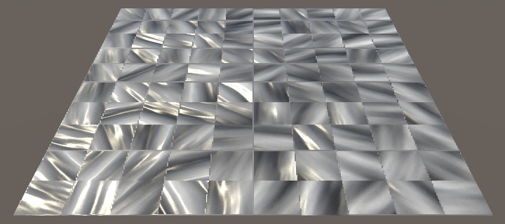
This doesn't entirely eliminate the problem, but makes it a lot less obvious.
Optional Mixing
Combining two grids is a lot more work than just using a single one. If the grid isn't obvious—for example because there aren't many specular reflections—then you might get away with a single grid. So let's make dual grids optional. This also makes it easier to compare both approaches. We'll make this possible by adding a toggle to our shader. This is an integer property with the Toggle attribute. This attribute requires a keyword as an argument, for which we'll use _DUAL_GRID.
		[NoScaleOffset] _FlowMap ("Flow (RG)", 2D) = "black" {}
		[Toggle(_DUAL_GRID)] _DualGrid ("Dual Grid", Int) = 0
		_Tiling ("Tiling, Constant", Float) = 1
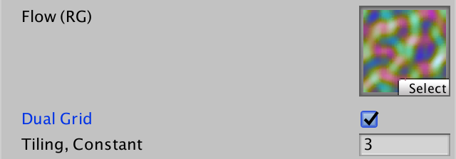
The integer portion of the property is not used by the shader, only the keyword matters. When the property is checked via the inspector, that keyword is defined, otherwise it isn't.
Add the #pragma shader_feature _DUAL_GRID statement to the shader, directly below the #pragma target 3.0 one. This instructs Unity to compile two variants of our shader. One with and one without the keyword enabled. Which one gets used depends on whether the material has the property checked.
		#pragma target 3.0

		#pragma shader_feature _DUAL_GRID

		#include "Flow.cginc"
The line of code that samples the second grid and averages both of them now has to only be included when the keyword is defined. That's done be enclosing it between pre-processor #if and #endif directives. The #if is followed by defined(_DUAL_GRID), which checks whether the keyword is defined. Only then will the code be included. This is a pre-processing step of the compilation process. One shader variant has that line of code in it, the other doesn't.
			float3 dh = FlowGrid(uv, time, false);
			#if defined(_DUAL_GRID)
				dh = (dh + FlowGrid(uv, time, true)) * 0.5;
			#endif
			fixed4 c = dh.z * dh.z * _Color;
Finally, remove the temporary scaling of the flow map.
float3 flow = tex2D(_FlowMap, uvTiled).rgb;
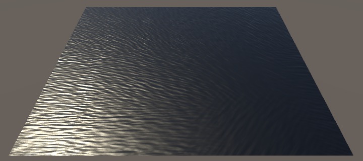
Dual grids also gives us a little more wiggle room when playing with the tiling scale.
The next tutorial is Waves.