Sine Waves
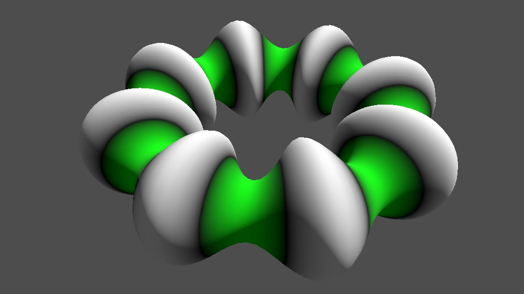
This is the first Godot tutorial in a series that covers the creation of procedural patterns on the GPU with shaders, using the Godot Engine, version 4.6.
It is assumed that you went through at least the first four parts of the Introduction series, or are familiar with Godot Engine 4 and have written a shader before.
At the bottom of my tutorials you'll find links to their license and an online repository containing the finished project.
Introduction
Surfaces are usually made with textures that are sampled in a shader, but procedural patterns are also useful. Procedural generation provides some benefits, like not needing textures, which both saves space and memory and also avoids slow memory access. There is no fixed resolution, which avoids blurry blocky textures, and obvious tiling from repeating textures can be avoided with non-repeating patterns. It is also possible to animate procedural patterns in more ways than just sliding or mixing textures.
There are also downsides to procedural patterns compare to sampling textures. The complexity of a pattern doesn't matter for a texture, but complex procedural patterns require more calculations. Texture aliasing can be mitigated with mip maps and filtering. Filtering can be done procedurally as well, but is more complicated and often requires evaluating the pattern multiple times. And because procedural patterns are purely computational there is no opportunity for the GPU to do other work at the same time, which it could do while waiting for a texture fetch to arrive, if warp occupancy is low enough. Also, complex surface shaders already perform a lot of lighting-related calculations, so the added work for a procedural pattern adds to that.
A hybrid approach of combining both textures and procedural patterns can aim to combine the strengths of both while covering for each other's weaknesses. Pure procedural patterns can be quite useful for special FX, especially when complex lighting is not needed. This series focuses on procedural patterns so uses them only.
Plane Scene
We start this series by creating a simple sine wave pattern. Once we can make good surfaces with waves we can move on to procedural noise patterns. We will start with 2D patterns, but because we'll apply them to 3D surface we'll put them in a 3D scene. We begin with the simplest surface, which is a flat plane.
Create a new Godot project with a 3D scene saved as sine_waves_plane.tscn
that has a Node3D root and a single MeshInstance3D child node named Plane
. Set its Mesh to a new PlaneMesh.
Set the plane's Geometry › Material Override to a new ShaderMaterial and set that material's Shader to a new shader. Select a normal shader with the spatial type and the default template and save it as sine_waves.gdshader
.
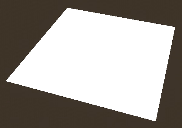
This gives us a minimal scene with a single white plane in it. We won't bother with setting up lights and a camera, relying on the default scene preview settings. If you want to run the scene as a standalone app you do have to set those up to see something useful.
I turned off the View Grid and View Origin toggles via the scene's View toolbar menu so the view is clear.
Coloring with UV
Open the shader in the Shader Editor. Delete all commented lines starting with //, only keeping the shader_type declaration and the empty vertex() and fragment() functions.
shader_type spatial;

void vertex() {}

void fragment() {}
We'll use the UV coordinates provided by the mesh to generate our pattern, like they're used to sample textures. To start things off let's directly use the UV coordinates for the red and green components of the surface color, leaving blue at zero. Because we're working with a spatial shader it calculates complex lighting in the 3D scene, so we do not simply set a color directly. Instead we'll set the surface albedo, which is defines its level of whiteness. This is done by assigning to ALBEDO in the fragment() function, which the built-in shader code of spatial shaders will use to determine how it appears when illuminated. It is an RGB color, the alpha channel is not part of it, so a vec3 can be directly assigned to it.
void fragment() {
	ALBEDO = vec3(UV, 0.0);
}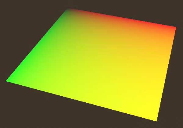
This shows us the UV layout on the plane. Without any rotation or scale the corner at (0,0) in the world XZ plane is black, the corner at (1,0) is red as the U coordinate is 1 there, likewise the corner at (0,1) is green, and the corner at (1,1) is yellow as both coordinates are 1 there. Note that the default plane has a size of 2×2 and its UV coordinates go from 0 to 1, so the 0–1 UV range is stretched across two units in the world XZ plane.
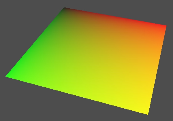
The color gradient created by the UV coordinates appears brighter than expected. This is because the spatial shader also adds environmental reflections to the surface. We can turn this off by disabling the preview environment via the scene's toolbar toggle button, which looks like a sphere wireframe. That lowers the brightness, replaces the background with solid gray, and makes it easier to see the pattern.
Sine Wave
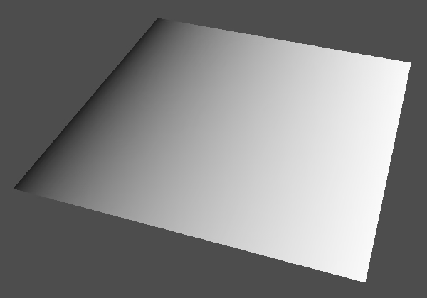
Instead of directly showing the UV coordinates we'll use them to sample a procedural pattern. The result is a single pattern sample that we use to create a color. So let's introduce a float pattern_sample variable and use that to fill a vec3 to create a grayscale color. We start very simple, by directly using the U coordinate for the pattern sample. This gives us a linear gradient in the U dimension, which matches the X dimension in world space because we haven't rotated the plane.
void fragment() {
	float pattern_sample = UV.x;
	ALBEDO = vec3(pattern_sample);
}
Color Perception
Our eyes are more sensitive to low light than bright light, meaning that we perceive greater differences between darker than between lighter colors. Thus the dark part of the gradient appears to change rapidly while the bright part appears mostly the same. We see the colors like this because Godot renders 3D scenes in linear color space, so the gradient is truly linear.
We could make the gradient appear linear to us by compensating for how we perceive it. A simple approximation would be to square the U coordinate.
float pattern_sample = UV.x * UV.x;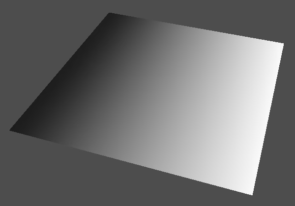
But we won't go into the details of color space and perception. It is sufficient to know that our perception is nonlinear. What we might intuitively think is 50% is actually roughly 25%, and what we might intuitively think is 70% is actually roughly 50%. This is usually not important but needs to be kept in mind when directly using values like UV coordinates and mathematical formulas for colors.
Producing a Wave
Having said that, we move on to finally showing a sine wave in the U dimension, by passing the U coordinate to the sin() function.
float pattern_sample = sin(UV.x);This won't appear to change the result much, because we end up showing only a part of the start of a wave. The sin() function can be interpreted as giving us one of the two coordinates of a 2D point while we travel along the circumference of a circle that has a radius of 1 unit. The cos() function gives us the other coordinate. Thus the result of the function oscillates between −1 and 1, producing a wave pattern, a single wave for going around the circle once.
Going around one full circle completes a single period of sin(). Thus the period of sin() is the same as the circumference of a circle with radius 1, which is 2π (two pi), or τ (tau) for short. So we create a full wave by multiplying τ and U and passing that to sin().
float pattern_sample = sin(TAU * UV.x);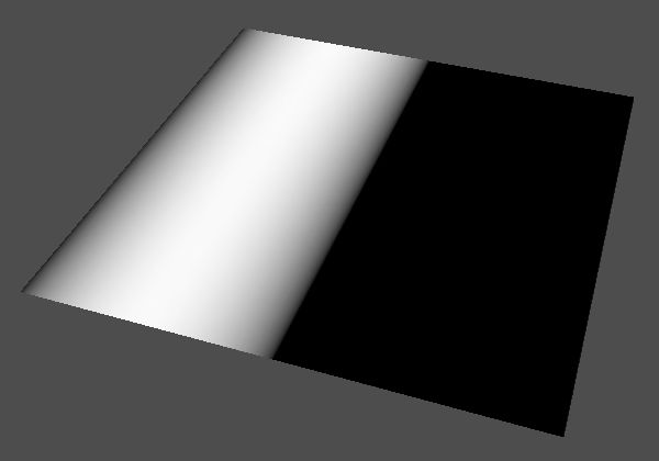
A sine wave starts at zero, then climbs to 1, drops back down to zero at the halfway point, then repeats in the opposite direction, going all the way to −1, then back to zero again. That completes a single period and one trip around the unit circle.
Colorizing the Wave
Negative colors end up as black, so the negative part of the wave appears solid black. We can make the entire wave visible by changing how we colorize it. First, let's give the colorizing code a dedicated colorize() function, which converts a given float value into a vec3 color.
vec3 colorize(float v) {
	return vec3(v);
}

void vertex() {}

void fragment() {
	float pattern_sample = sin(TAU * UV.x);
	ALBEDO = colorize(pattern_sample);
}
Then we change colorize() to convert the pattern's −1–1 range to 0–1, by halving it and adding ½.
vec3 colorize(float v) {
	return vec3(v * 0.5 + 0.5);
}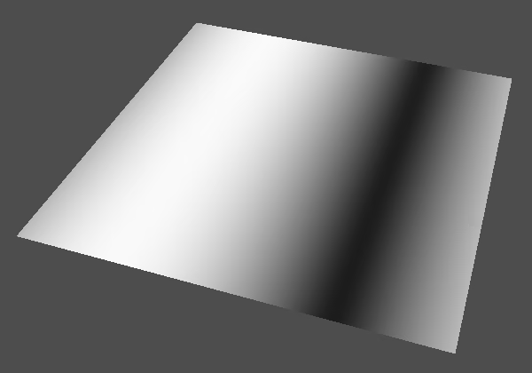
We can now see the entire wave, but it is hard to interpret because we do not perceive colors linearly. So let's change our approach, keeping the wave centered on zero and instead making the negative part positive, by taking the absolute of the value, using abs().
return vec3(abs(v));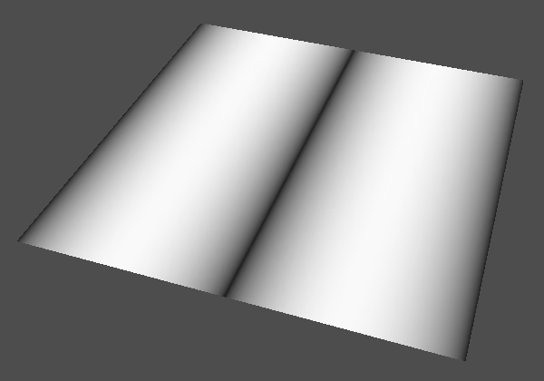
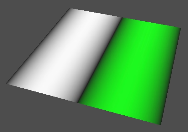
This works, but we can no longer distinguish between the positive and negative parts of the wave. So let's go a step further and change the color for the negative part to green. Replace the single return statement with with an if–else choice, returning the value as a grayscale color if it is at least zero, otherwise using the negated value for the green color component only.
vec3 colorize(float v) {
	if (v >= 0.0) {
		return vec3(v);
	}
	else {
		return vec3(0.0, -v, 0.0);
	}
}
Shouldn't we avoid branching in shaders?
While no longer an iron-clad rule, that is generally good advice, although there are different kind of branches to consider. However, the shader code that we write is far removed from the instructions that end up being executed by the GPU. I write a verbose if–else block for clarity, but it could be condensed to:
if (v >= 0.0) {
	return vec3(v);
}
return vec3(0.0, -v, 0.0);
It could be condensed further to a single ternary operation:
return v >= 0.0 ? vec3(v) : vec3(0.0, -v, 0.0);All three ways of writing it would most likely end up as the same GPU instructions, using conditional assignments instead of a branch. This makes it harder to predict what a GPU actually does but allows us to write more readable code.
Sampling per Vertex
We are currently sampling the pattern per fragment, but it is also possible to sample it per vertex instead. Let's see what that looks like.
We keep the code that samples per fragment in place, so move the pattern sampling code to its own sample_pattern() function. Because UV is only available inside fragment() and vertex() we have to add a parameter for the coordinates.
float sample_pattern(vec2 uv) {
	return sin(TAU * uv.x);
}

void vertex() {}

void fragment() {
	float pattern_sample = sample_pattern(UV);
	ALBEDO = colorize(pattern_sample);
}
Then also sample the pattern in vertex(), passing it the vertex UV. Colorize the result and assign it to the RGB components of the vertex COLOR, replacing the default vertex color.
void vertex() {
	float pattern_sample = sample_pattern(UV);
	COLOR.rgb = colorize(pattern_sample);
}
Next, use COLOR in fragment() to set ALBEDO. Keep the existing ALBEDO in place and put the new assignment after it. That will replace the per-fragment sample. Shader compilers will detect this and omit all unused code, so the pattern will not be evaluated per fragment anymore even though the code is still in place.
void fragment() {
	float pattern_sample = sample_pattern(UV);
	ALBEDO = colorize(pattern_sample);
	ALBEDO = COLOR.rgb;
}
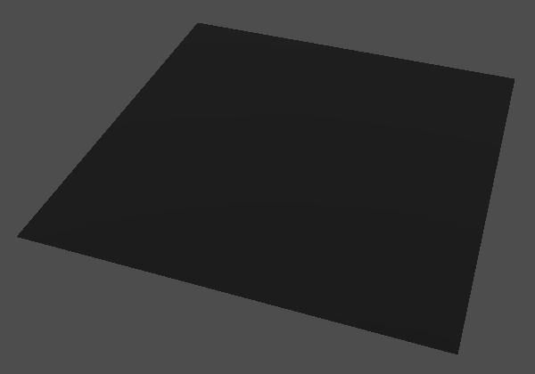
The result is a solid black plane.
Plane Vertices
We get this result because the default plane is a mesh with only four vertices at its corners. So we sample only at those points and our wave is zero at all of them. The vertex data gets linearly interpolated across the triangles that make up the mesh's surface. So we end up interpolating between only black. We can see this by changing from Display Normal to Display Wireframe via the scene view's Perspective dropdown menu.
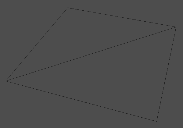
So sampling per vertex means that we're severely undersampling our pattern. We can improve this by increasing the vertex density of our place, increasing its Subdivide Width and Subdivide Depth, which are set to zero by default. Let's set both to 8.
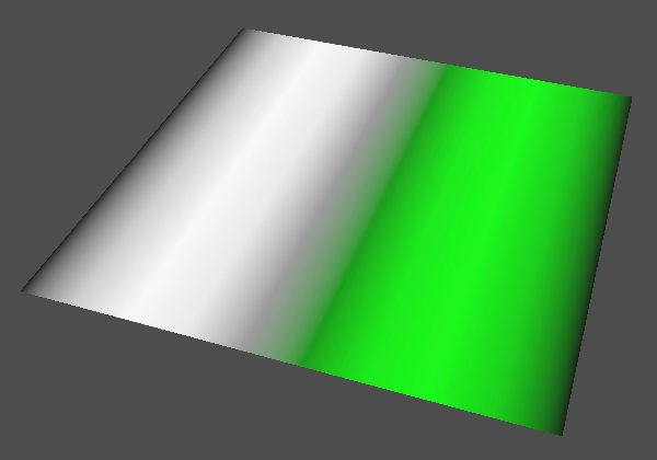
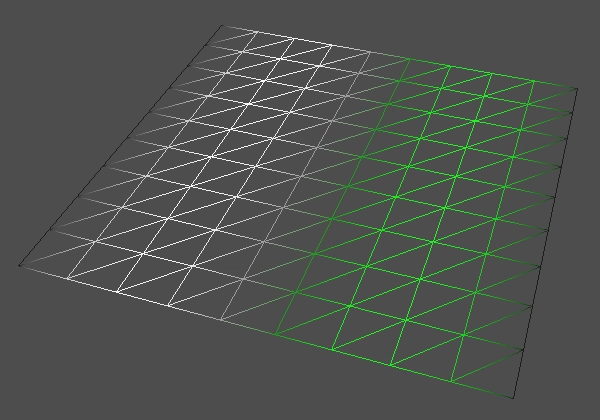
Now we see the sine wave again, but it looks ugly because we use only ten sampling points: the two vertices at the edges of the plane plus eight more in between. The color gets linearly interpolated in between those points, which at this subdivision level is a poor approximation of the wave.
The ugliest part is the middle, because we end up interpolating from gray to green, missing the full black where the waves is zero. We can improve that by increasing the subdivision to 9, because then we get a vertex exactly in the middle of the wave. So it's not just important how often we sample, but also where we sample, which depends on the pattern.
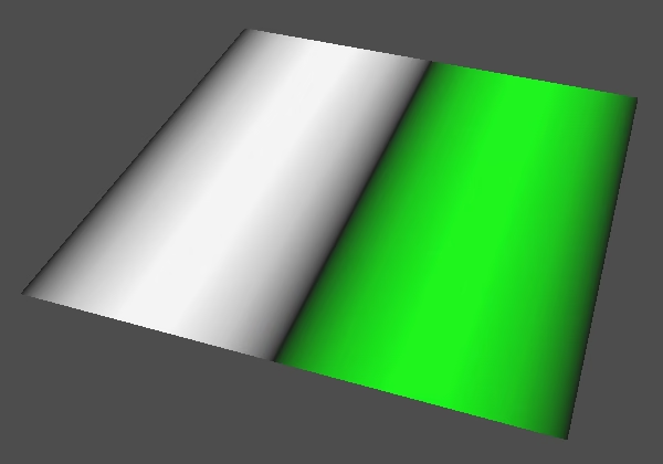
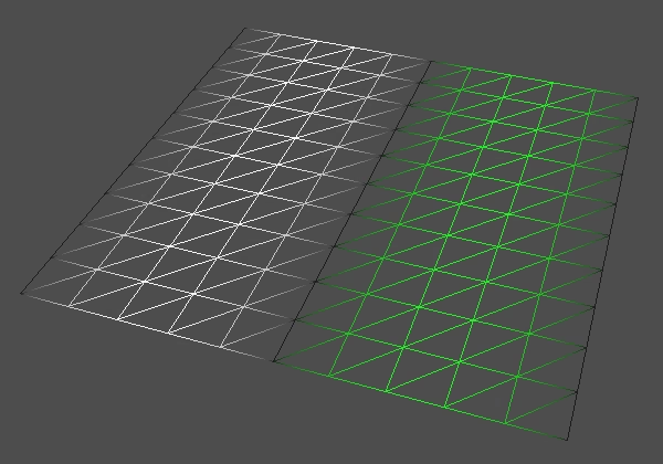
Sampling the pattern per vertex means that we can avoid doing it per fragment, but it also means that we undersample the pattern, which affects its quality. So it is a trade-off.
Vertex Offset
Sampling per vertex also gives us the opportunity to change the position of the vertex. This allows us to use the pattern to vertically offset the plane. We do this by adjusting the Y component of VERTEX. Let's add the pattern sample to it. This adjust the vertex positions in object space, so no matter how it is transformed it will look like a sine wave.
void vertex() {
	float pattern_sample = sample_pattern(UV);
	COLOR.rgb = colorize(pattern_sample);
	VERTEX.y += pattern_sample;
}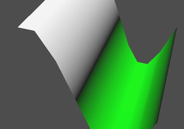
Our plane now curves its surface to match the pattern. As this is done per vertex we're still undersampling, so the surface is approximated with linear segments.
Modulated Displacement
Our wave is currently rather steep. We typically don't want such a large displacement, so let's make it configurable. Add a uniform float displacement variable to the shader, set to 0.2 by default. This adds a Displacement property to our material's Shader Parameters inspector section. Let's add hint_range(-1.0, 1.0) so it is easy to adjust via a slider. We set its minimum to −1 so it is possible to invert the displacement.
shader_type spatial;

uniform float displacement : hint_range(-1.0, 1.0) = 0.2;
Use the displacement to scale the pattern sample when adjusting the vertex position.
VERTEX.y += pattern_sample * displacement;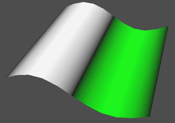
Wave on a Torus
We're not limited to applying our pattern to just a plane, so let's introduce another shape. We pick a torus, because it has an interesting curved surface that has an UV space that forms a closed loop.
Duplicate our scene and rename the new one to sine_waves_torus.tscn
. Rename its MeshInstance3D node to Torus
and set its mesh to a TorusMesh. We'll keep the default settings of this mesh.
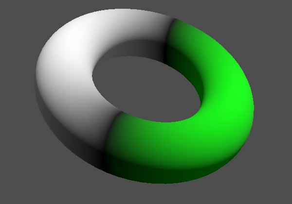
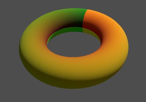
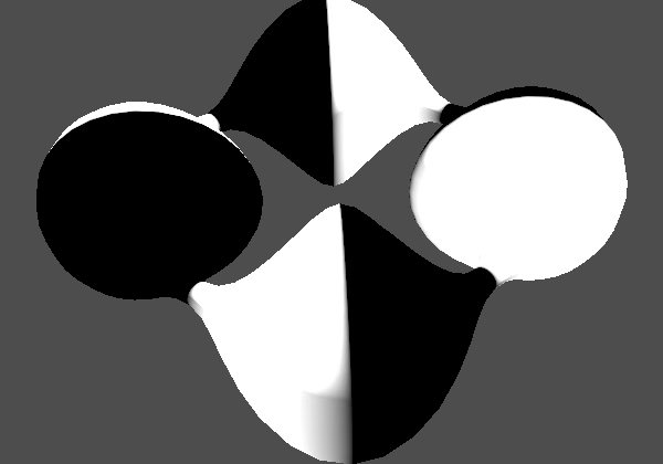
Our wave ends up wrapped around the torus counterclockwise, which makes its left half white and its right half green. Its left half is displaced upward and its right half is displaced downward. But because the wave wraps around the ring-shaped surface of the torus it would make more sense to displace it outward and inward instead. That way the ring would get thicker and thinner.
We can make the displacement relative to the surface by offsetting along its normal vector. The normal vector is a vector with length 1 that points straight away from the surface, defining a local up direction for anything that would stand on that surface. In the case of our plane its normal vector simply points up, matching the Y axis in its object space. This means that we could rewrite our vertex displacement so it adds the scaled (0,1,0) vector to VERTEX instead of adding to its Y component only.
VERTEX += vec3(0.0, 1.0, 0.0) * (pattern_sample * displacement);This will produce exactly the same result as before and would likely compile to the exact same GPU instructions. But now we replace the constant vector with the mesh's normal vector that is defined per vertex, accessed via NORMAL.
VERTEX += NORMAL * (pattern_sample * displacement);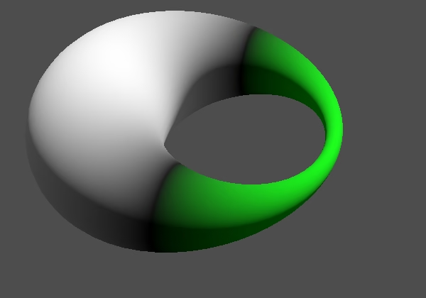
Our plane is still the same, but our torus now gets thicker on its left side and thinner on its right side. The deformation is pronounced, because the default torus has an inner radius of 0.5 and an outer radius of 1, so the ring of the torus has a diameter of 0.5 and thus a radius of 0.25. The displacement adjust that last radius. So with Displacement set to 0.2 the ring's radius varies between 0.45 and 0.05.
Wave Frequency
We're not limited to showing only a single period of a sine wave, we can repeat it. How often a wave repeats is defined by its frequency. Frequency usually represents how often something repeats per second, but in our case it will represent how often the wave repeats per unit of whatever we pass to the sample_pattern() function, which is currently U.
Add a uniform float frequency variable to the shader, set to 1 by default. We won't constrain it and it could even be negative, which would reverse the pattern.
uniform float displacement : hint_range(-1.0, 1.0) = 0.2;
uniform float frequency = 1.0;
The frequency is applied by using it to scale what we pass to sin().
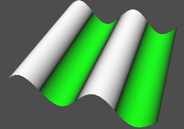
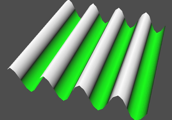
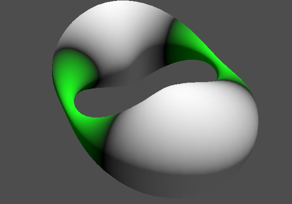
return sin(frequency * TAU * uv.x);Increasing the frequency makes the pattern change faster, which makes the quality degradation from sampling per vertex worse. So let's increase the plane subdivisions to 31. Then try frequency 2 and 4.
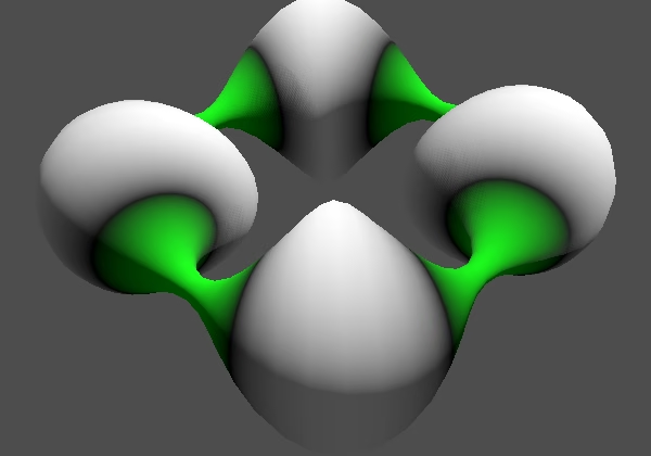
Surface Normal Vector
Although we deform the surfaces of our plane and torus the shader still applies lighting to them as if they were unmodified. That's because the orientation of the surface used for lighting calculations is represented by its normal vectors, which we do not modify. Shadows cast and received by the surfaces is correct because that depends on the vertex positions, which we do modify. But besides that the shading of the surfaces does not match their deformed shapes.
We can see this by setting ALBEDO to NORMAL in fragment(). That's the interpolated vertex normal, renormalized so its length is 1 after interpolation.
	ALBEDO = COLOR.rgb;
	ALBEDO = NORMAL;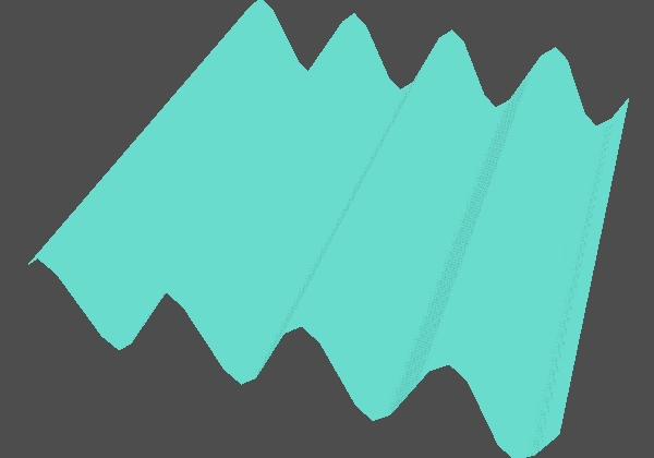
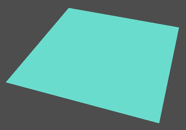
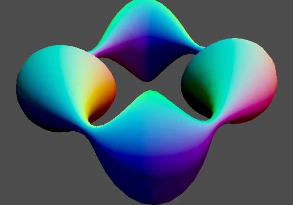
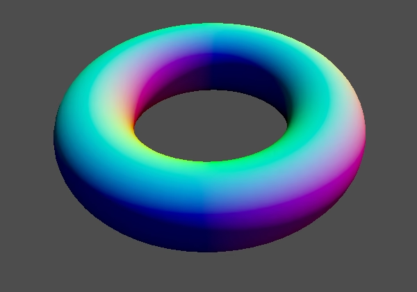
This shows us the normal vectors as colors. Note that the fragment normal is in view space, so the colors we see depend on the view angle.
Pattern Sample with Derivative
To provide normal vectors that match the deformed surface we have to not only produce a single value per pattern sample but also something that describes the shape of the surface of the function. We can do this by including the slope of the curve described by the function at that point. We do this by including its rate of change. For example, if the function were simply U then its rate of change would be 1. In general the rate of change of a function is described by its derivative function.
So a pattern sample does not only have a value but also a derivative. Let's formalize this by introducing a custom PatternSample struct type that contains two float fields: v for its value and d for its derivative. Make sample_pattern() return that, initially with the derivative set to zero. We can create a struct value via a constructor function named after its type, with arguments matching the order of its fields.
struct PatternSample {
	float v;
	float d;
};

PatternSample sample_pattern(vec2 uv) {
	return PatternSample(
			sin(frequency * TAU * uv.x),
			0.0
	);
}
Can't we just use vec2?
Yes, and it would be equivalent, there is no difference in the GPU instructions. Using vec2 provides no performance benefit here because the shader compiler is free to arrange things optimally, without being constrained to predefined vector types. Also, if we end up using only one of the fields the other would be entirely eliminated by the compiler. So I prefer the approach with clearer semantics.
Adjust vertex() and fragment() so they work with PatternSample. Then use the derivative to set ALBEDO. This will make our surfaces solid black.
void vertex() {
	PatternSample pattern_sample = sample_pattern(UV);
	COLOR.rgb = colorize(pattern_sample.v);
	VERTEX += NORMAL * (pattern_sample.v * displacement);
}

void fragment() {
	PatternSample pattern_sample = sample_pattern(UV);
	ALBEDO = colorize(pattern_sample.v);
	ALBEDO = COLOR.rgb;
	ALBEDO = NORMAL;
	ALBEDO = vec3(pattern_sample.d);
}
Wave Derivative
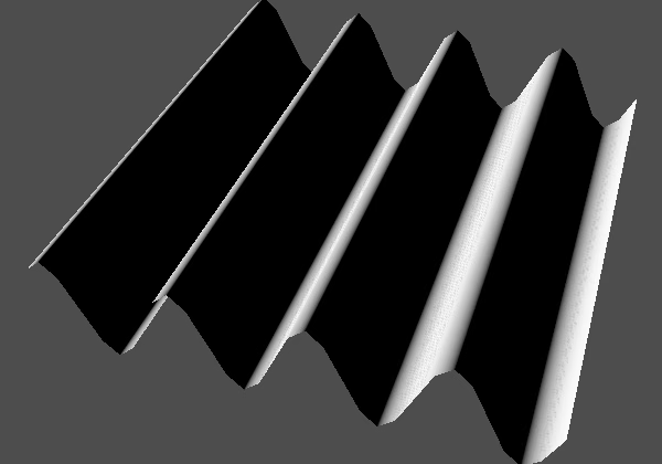
The derivative of sin() is simply cos(), which is the same function shifted forward by a quarter of its period.
PatternSample sample_pattern(vec2 uv) {
	return PatternSample(
			sin(frequency * TAU * uv.x),
			cos(frequency * TAU * uv.x)
	);
}
Repeating the exact same code won't result in duplicated GPU work, because shader compilers recognize this and will ensure that the work is only done once. However, in this case it is more convenient to also write it only once, so let's store what we pass to sin() and cos() in a variable t. This will produce the exact same GPU instructions.
PatternSample sample_pattern(vec2 uv) {
	float t = frequency * TAU * uv.x;
	return PatternSample(
			sin(t),
			cos(t)
	);
}
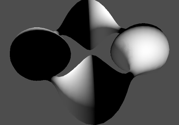
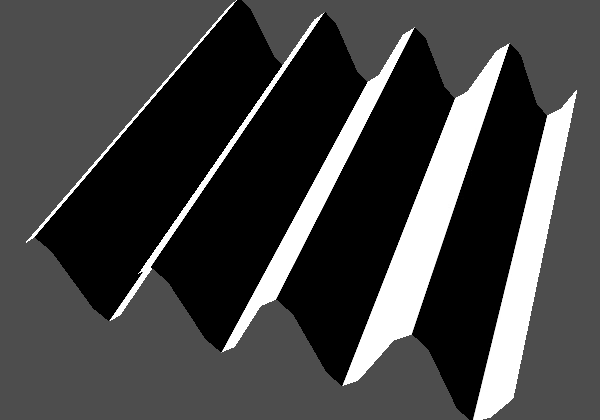
However, derivatives are more complicated than that. We're not just passing U directly to sin(), we scale it. For example, if we double U first then the wave changes twice as fast. Passing the same to cos() makes it change twice as fast to match, but the rate of change it represents should be doubled as well, because the curve has become twice as steep. Hence we should double the derivative. So in general we have to scale the derivative by the frequency, incorporating τ into it for convenience. This can be done easily by introducing a variable f for it.
PatternSample sample_pattern(vec2 uv) {
	float f = frequency * TAU;
	float t = f * uv.x;
	return PatternSample(
			sin(t),
			f * cos(t)
	);
}
Tangent and Normal Vectors
Now that we have correct derivatives we can turn them into vectors. The derivative represents the rate of change, in our case the rate of change per unit of U. We can use this to make a vector that points in the direction of change, tangential to the surface. For a flat plane without displacement that would simply be (1,0,0), which is its current tangent vector. To make it follow the surface we have to change it to (1,d,0) where d is the derivative. Let's use that for ALBEDO.
ALBEDO = vec3(1.0, pattern_sample.d, 0.0);Like the normal vector the tangent vector should have length 1, which is only the case when there is no displacment. So we normalize the vector, by passing it through the normalize() function.
ALBEDO = normalize(vec3(1.0, pattern_sample.d, 0.0));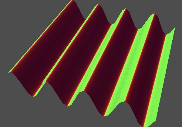
This shows us the tangent vectors for the displaced plane, in object space. The tangent and normal vectors are perpendicular. The tangent vector points along the surface while the normal vector points away from it. We go from tangent to normal by rotating the tangent upward by 90 degrees, around the V axis. This is effectively a 2D rotation, which we can do by swapping X and Y and negating X.
ALBEDO = normalize(vec3(-pattern_sample.d, 1.0, 0.0));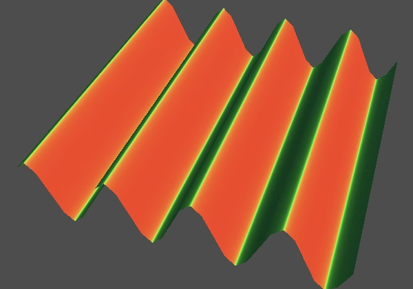
Normal Vectors for Plane
This gives us normal vectors that match our pattern, but not the actual displacement, because we modulate that via the Displacement property. So the derivative value that we use must be scaled by that as well. Let's put it in a separate variable d.
	float d = pattern_sample.d * displacement;
		ALBEDO = normalize(vec3(-d, 1.0, 0.0));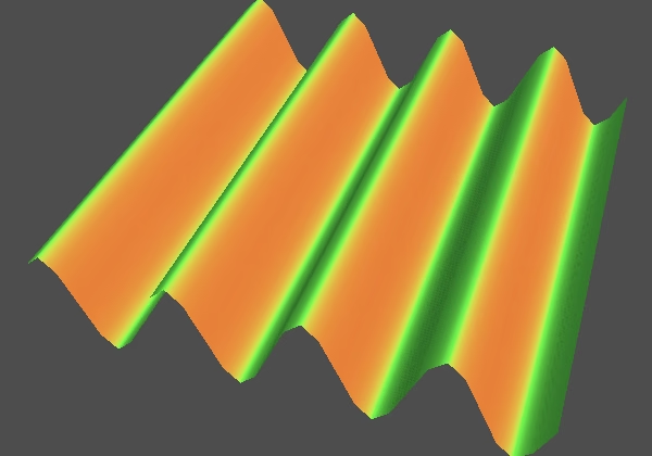
These normals better match the visible surface, but still not exactly. We assume that one unit in UV space corresponds to one unit in 3D world space. This is not the case for our plane, because it is two units wide, which is its default Size. If we reduced it to 1 then the normals would be correct. However, we keep it at its current size and instead add a uniform float bumpiness variable to our shader to tweak how displaced it appears. We set it to 1 by default but then set its material property to 0.5 to get correct normals for the plane.
uniform float bumpiness = 1.0;
uniform float displacement : hint_range(-1.0, 1.0) = 0.2;
Factor bumpiness into d to produce the desired normal vector.
	float d = pattern_sample.d * displacement * bumpiness;
	ALBEDO = normalize(vec3(-d, 1.0, 0.0));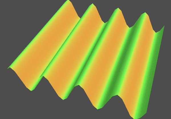
We do it like this because there are lots of intricacies involved with getting the correct normals, including the mesh's transformation and UV mapping, but that's not the focus of this series. We instead make it manually adjustable, which also allows for artistic choices that might be more visually pleasing or interesting than being physically correct.
Normal Vectors in General
Our current approach only works for the plane and only when it is not rotated. To generalize our approach we have to replace the simple rotation of the tangent with a cross product. The cross product of two 3D vectors produces another vector that is perpendicular to both. So if we take the cross product of the X and Z axes we get the Y axis. In our case, the cross product of the tangent vector for U and the tangent vector for V gives us the normal vector.
For a flat plane this means that (1,0,0)✗(0,0,1) gives us (0,1,0). Actually, it'll give us (0−1,0), so we'll negate the second vector to flip the sign. We perform the cross product with cross(), using our tangent vector for its first argument.
	ALBEDO = normalize(cross(
			vec3(1.0, d, 0.0),
			vec3(0.0, 0.0, -1.0)
	));
This produces the exact same result as our manual rotation earlier. We can go a step further and split the tangent vector in two parts: the unmodified flat tangent vector plus a vector with only d for its Y component.
	ALBEDO = normalize(cross(
			vec3(1.0, 0.0, 0.0) + vec3(0.0, d, 0.0),
			vec3(0.0, 0.0, -1.0)
	));
Which means that we add the normal vector of the plane scaled by the derivative to the tangent vector. Writing it like that still produces the exact same result.
	ALBEDO = normalize(cross(
			vec3(1.0, 0.0, 0.0) + vec3(0.0, 1.0, 0.0) * d,
			vec3(0.0, 0.0, -1.0)
	));
Now we can generalize to any surface, by using the unmodified TANGENT and NORMAL vectors of the fragment. We have to use the tangent vector for V as well, which is know as the BINORMAL.
	ALBEDO = normalize(cross(
			TANGENT + NORMAL * d,
			BINORMAL
	));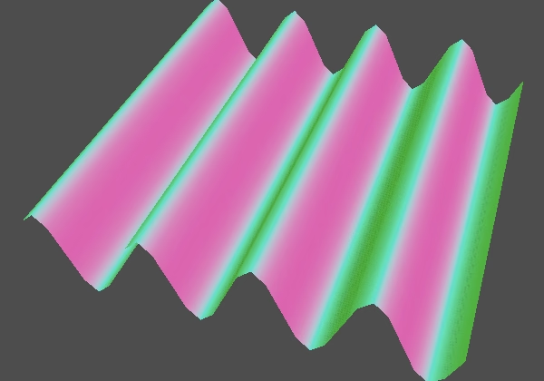
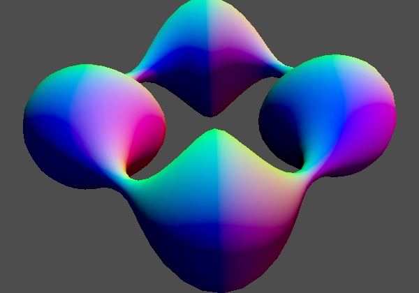
The normal vector that we get out of this is in view space and it also looks plausible for the torus. It is only partially correct though, because we do not take the original curvature of the torus into account. Just like scaling the input to a function changes its derivative, so does wrapping it around a curved surface, because then displacement also effectively scales it. However, if the displacement is small this error is not something anyone would notice. The 0.2 displacement is fairly large thus the error is large as well, but I keep it at that amount to make the deformation clearer.
What bumpiness is correct for the torus? Because it isn't flat the right bumpiness value varies across its surface and with the applied displacement. On the outside of the torus pushing the surface outward scales it up, while on the inside of the torus pushing the surface outward scales it down. Both should affect the derivatives, but we'll ignore that for simplicity. While we could calculate correct derivatives for the torus, in general the pattern can be wrapped around any arbitrary surface and we have no idea how to make it perfect. So we'll just pick a reasonable bumpiness.
Our torus has a minor radius of 0.5 and a major radius of 1.0. So the ring it forms envelops a circle with radius 0.75, which has circumference ¾τ. The U dimension wraps around that, so that's how stretched U is on average. So let's set its bumpiness to 1 divided by that, which is roughly 0.212. This is never correct, but equally distributes the error.
Shaded Surfaces
Now that we have decent normal vectors show the vertex colors again so we can see our surfaces both colored and shaded.
	ALBEDO = COLOR.rgb;
	//ALBEDO = NORMAL;
	float d = pattern_sample.d * displacement * bumpiness;
	NORMAL = normalize(cross(
			TANGENT + NORMAL * d,
			BINORMAL
	));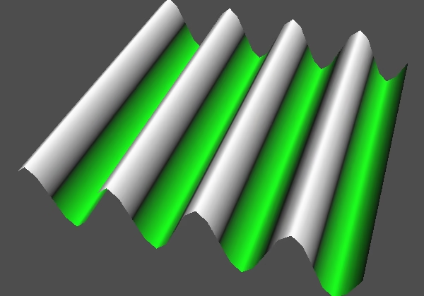
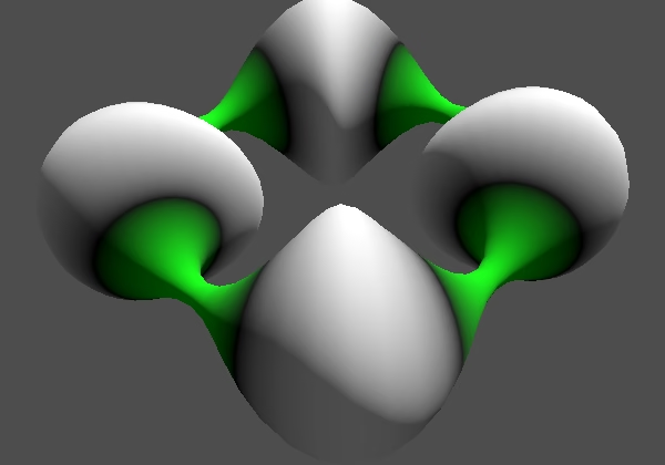
Finally, the spatial shader already normalizes NORMAL itself after we set it, so we don't have to do it ourselves.
	NORMAL = cross(
			TANGENT + NORMAL * d,
			BINORMAL
	);
The next tutorial is 2D Waves.