2D Waves

The Other Dimension

In the first tutorial we only used the U coordinate to sample our sine wave pattern, which effectively makes it a 1D pattern, even though we use it to alter a 3D shape. As we're using the UV coordinates to sample the pattern we also have a second dimension to play with.

Let's begin by replacing the U coordinate with the V coordinate in sample_pattern() and see how that looks.

	float t = f * uv.y;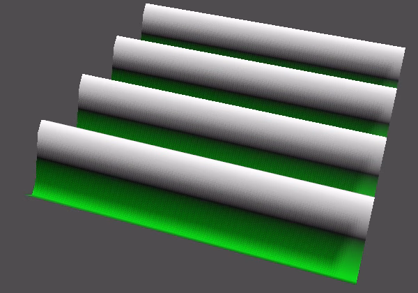

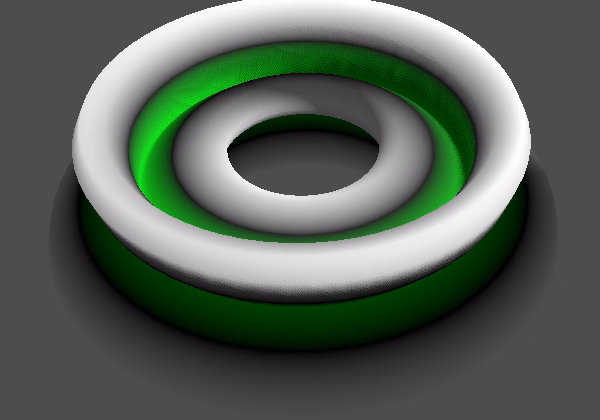
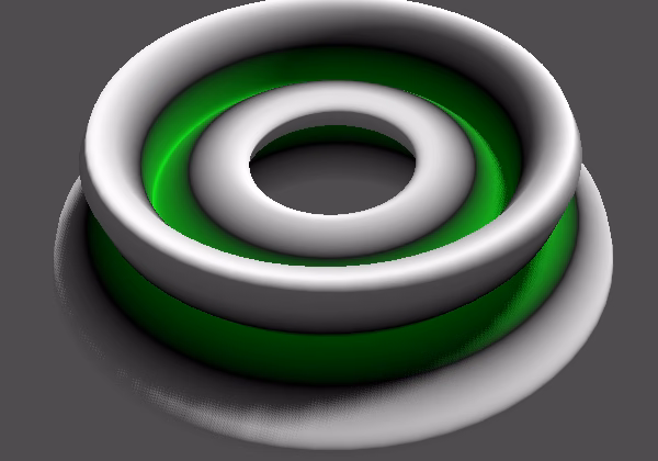
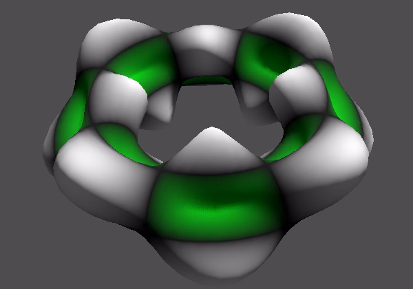
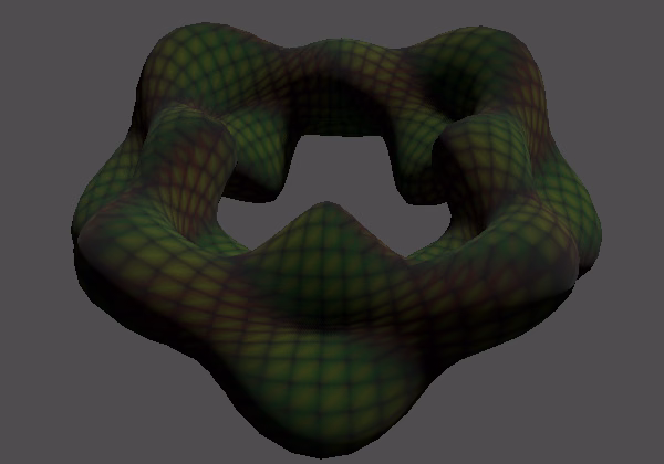
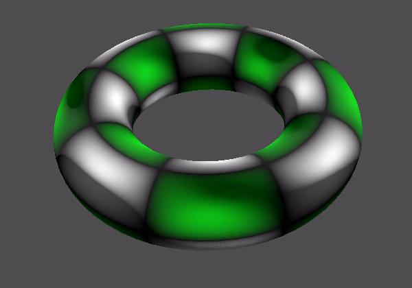
This produces alternative waves. In the case of the plane the orientation of the waves changed as if the pattern was rotated 90°. The difference is more pronounced for the torus, because the pattern now wraps around the minor radius, going around its ring from inside to outside and back again, instead of wrapping around the ring's loop.

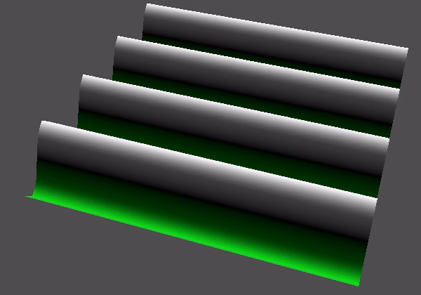
Normal Vectors for V

The normals vectors are now wrong, because we assumed that they were for a function in the U dimension, which is no longer the case. Now BINORMAL has to be adjusted instead TANGENT. Also, because the binormal is negative we have to subtract from it instead of adding to it.

	NORMAL = cross(
			TANGENT, // + NORMAL * d,
			BINORMAL - NORMAL * d
	);

That fixed the normal vectors. But for the torus the V dimension is stretched less than the U dimension. V is wrapped around the circumference of the ring on average, which has a diameter of 0.5, so we set its bumpiness to one divided by 0.5τ, which is roughly 0.637.

Both Dimensions

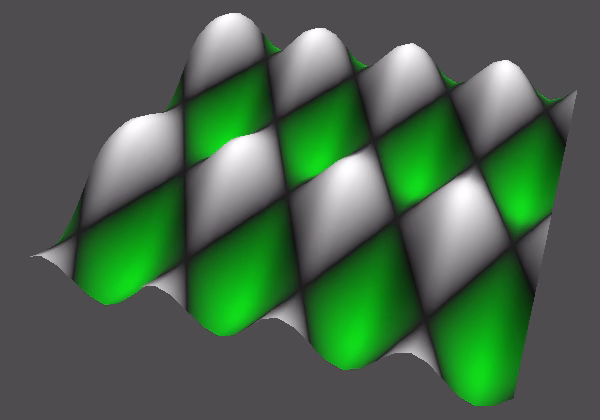
The next step is to use both dimensions to sample the pattern. The most straightforward way to do this would be to add U and V and pass that to sin(), but that would simply produce a diagonal wave. It is more interesting to create two waves, one per dimension, and then combine them. So let's do that and average both waves, adding them together and halving them, so the range of our pattern remains the same.

Change the t variable to a vec2 and pass it to sin() twice for both dimensions, then average the result. We'll ignore the derivative for now, keeping it the same.

PatternSample sample_pattern(vec2 uv) {
	float f = frequency * TAU;
	vec2 t = f * uv;
	return PatternSample(
			(sin(t.x) + sin(t.y)) * 0.5,
			f * cos(t.x)
	);
}

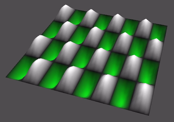
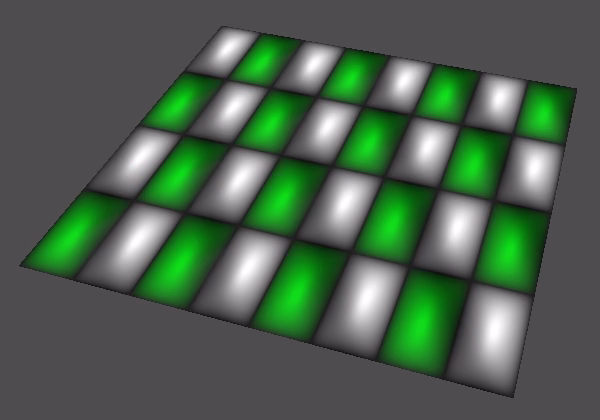
Let's set the displacement to zero for a moment so we can see the color pattern better on the plane.

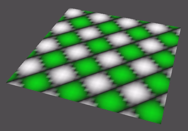
This produces a rotated checker pattern or diamond pattern. But because we're sampling per vertex the black lines along one of the diagonals degenerates into dotted lines and the result doesn't look good overall. So let's switch back to sampling the color per vertex, by removing the assignment of the interpolated vertex color to ALBEDO in fragment().

	ALBEDO = colorize(pattern_sample.v);
	//ALBEDO = COLOR.rgb;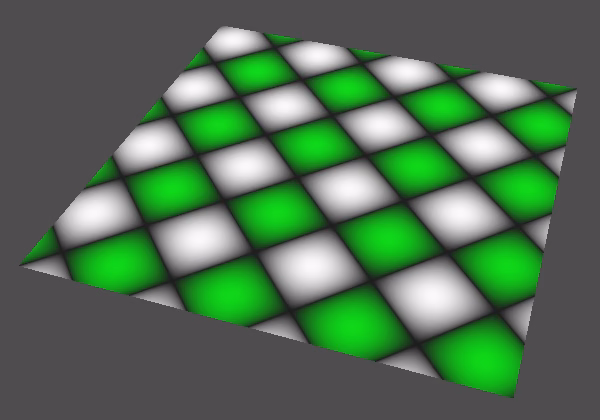

Independent Frequencies

We are not limited to using the same frequency for both waves; we can use separate frequencies for U and for V. To support that we change the frequency variable to a vec2.

uniform vec2 frequency = vec2(1.0);

Adjust sample_pattern() so it works with separate frequencies.

	vec2 f = frequency * TAU;
	vec2 t = f * uv;
	return PatternSample(
			(sin(t.x) + sin(t.y)) * 0.5,
			f.x * cos(t.x)
	);

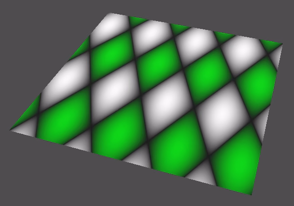
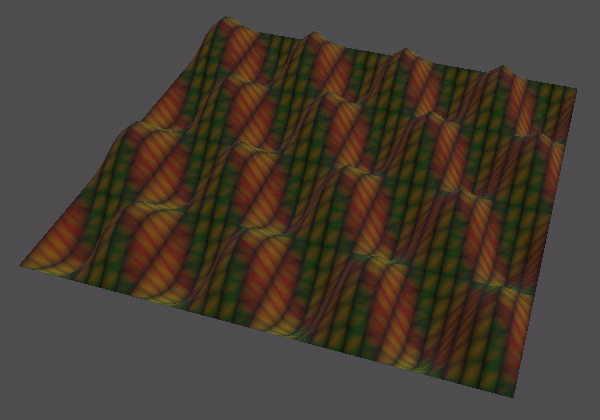
This allows us to deform the pattern so it is no longer square. Conversely, it allows us to compensate for unequally stretched UV dimensions, like for the torus.

Partial Derivatives

Because we changed our function we also have to change its derivative function to match. Currently the derivative that we calculate is still for a simple sin() in the U dimension. But we're now adding a second wave based on V and halving the result.

Halving the result is simple, that's just another scale that we have to apply to the derivative.

	return PatternSample(
			(sin(t.x) + sin(t.y)) * 0.5,
			f.x * cos(t.x) * 0.5
	);

That gives us the correct derivative for the U dimension. Because V is constant in the U dimension it doesn't change, so its derivative is zero. But that is only half of the derivative, because we must also include the rate of change in the V dimension. So we have two independent derivatives, one per dimension. These are the partial derivatives for U and V.

We need two derivatives, so change the d field of PatternSample to a vec2.

struct PatternSample {
	float v;
	vec2 d;
};

Then assign a vec2 to it in sample_pattern(), with the derivative for U that we already have. The derivative for V is the same, but with V instead of U.

PatternSample sample_pattern(vec2 uv) {
	vec2 f = frequency * TAU;
	vec2 t = f * uv;
	return PatternSample(
			(sin(t.x) + sin(t.y)) * 0.5,
			vec2(
					f.x * cos(t.x) * 0.5,
					f.y * cos(t.y) * 0.5
			)
	);
}

To get correct normals we have to apply both derivatives in fragment(), using the U derivative to adjust TANGENT and the V derivative to adjust BINORMAL.

	vec2 d = pattern_sample.d * displacement * bumpiness;
	NORMAL = cross(
			TANGENT + NORMAL * d.x,
			BINORMAL - NORMAL * d.y
	);

We should also support bumpiness per dimension, so change bumpiness to a vec2 as well. Then we can set it to (0.5,0.5) for the plane and (0.212,0.637) for the torus.

uniform vec2 bumpiness = vec2(1.0);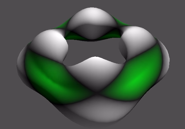

Alternative Functions

Let's adjust our shader so it can produce different patterns. Add a uniform int function variable to it, set to zero by default. Give it the hint_enum() hint so it becomes a dropdown selection list in the material's inspector, based on the list of strings that we give it. Let's use "U", "V", "UV Average", matching the three functions that we have produced so far.

uniform vec2 frequency = vec2(1.0);
uniform int function : hint_enum("U", "V", "UV Average") = 0;

We now have to change approach depending on function in sample_pattern(), with 0, 1, and 2 representing the three options. To make our code a bit more compact we'll first declare a PatternSample s variable, then set its fields and sub-fields, and then return it.

PatternSample sample_pattern(vec2 uv) {
	vec2 f = frequency * TAU;
	vec2 t = f * uv;
	PatternSample s;
	s.v = (sin(t.x) + sin(t.y)) * 0.5;
	s.d.x = f.x * cos(t.x) * 0.5;
	s.d.y = f.y * cos(t.y) * 0.5;
	return s;
}

Then we introduce a switch block, which gets case labels for the functions that we support. We start with all cases producing the same current pattern, which is the UV average pattern. At the end of that case we have to break to indicate that it ends there.

PatternSample sample_pattern(vec2 uv) {
	vec2 f = frequency * TAU;
	vec2 t = f * uv;
	PatternSample s;
	switch (function) {
		case 0: // U
		case 1: // V
		case 2: // UV Average
			s.v = (sin(t.x) + sin(t.y)) * 0.5;
			s.d.x = f.x * cos(t.x) * 0.5;
			s.d.y = f.y * cos(t.y) * 0.5;
			break;
	}
	return s;
}

At this point picking another function makes no different yet. So work out the cases for the separate U and V functions, each with their own break, otherwise they would roll over to the next case.

		case 0: // U
			s.v = sin(t.x);
			s.d.x = f.x * cos(t.x);
			s.d.y = 0.0;
			break;
		case 1: // V
			s.v = sin(t.y);
			s.d.x = 0.0;
			s.d.y = f.y * cos(t.y);
			break;
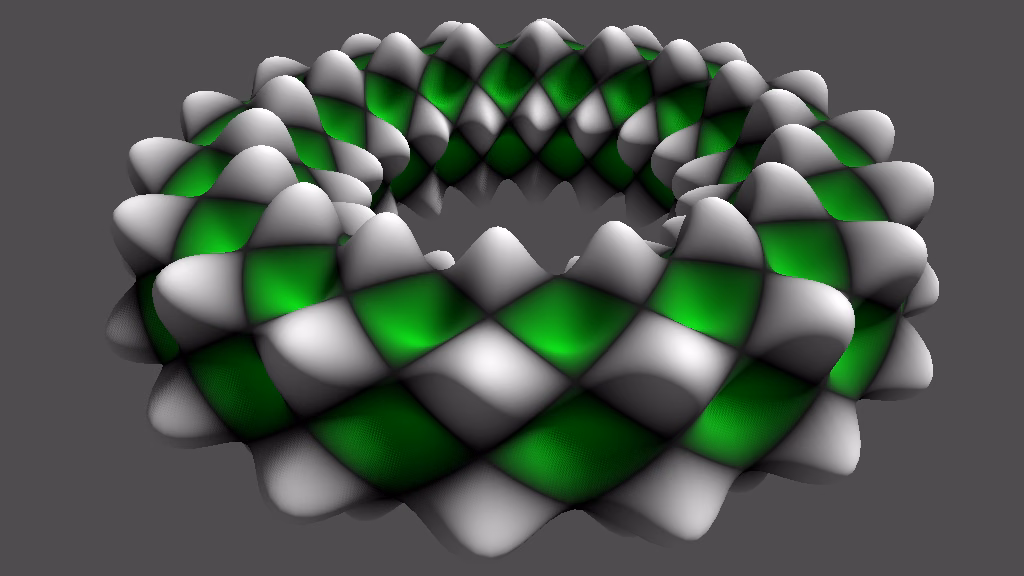
		case 2: // UV Average

Wave Product

Let's add a fourth function: the UV product, which multiplies the U and V waves instead of averaging them. It will produce a checker pattern that isn't rotated. Include it in the function hint.

uniform int function : hint_enum("U", "V", "UV Average", "UV Product") = 0;

And add a case for it in sample_pattern. Let's leave the derivatives at zero for now.

		case 3: // UV Product
			s.v = sin(t.x) * sin(t.y);
			s.d.x = 0.0;
			s.d.y = 0.0;
			break;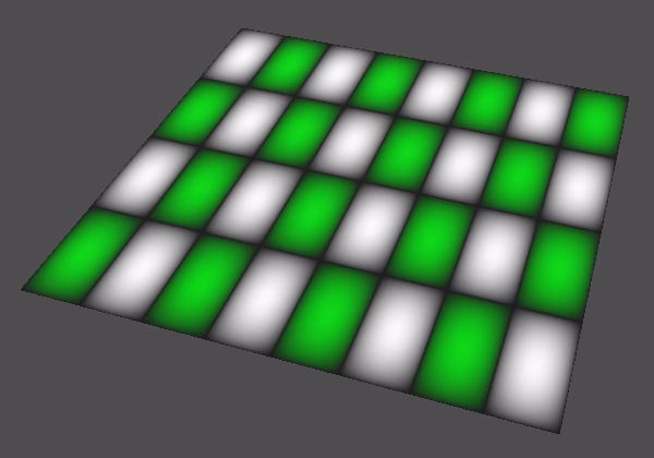

The partial derivatives of this function are found the same way as before, but now we have to include the value of the other dimension, because it scales the result. So we end up using the same sin() values twice. We could store those in variables, but that doesn't add much clarity here so I just repeat the code; the shader compiler will avoid the repetition.

			s.v = sin(t.x) * sin(t.y);
			s.d.x = f.x * cos(t.x) * sin(t.y);
			s.d.y = f.y * sin(t.x) * cos(t.y);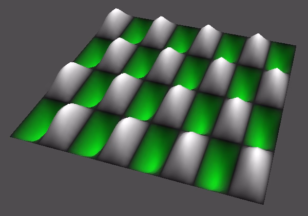

Using Vertex Data

Our shader has become a miniature uber shader, supporting different functions. If you'd only need a single function then it's best to turn function into a constant value, which would eliminate all unused code and avoid the uniform branching of the switch. But because our shader is for demonstration purposes we keep it flexible.

We can take this uber shader approach a step further and add more options to it. Let's make it configurable whether it samples colors per vertex or per fragment, because that can make a big difference and it's convenient to be able to compare both approaches.

Add a uniform bool color_per_vertex variable to the shader that is set to false by default so we get colors per fragment. This will become a toggle option in the material inspector.

uniform int function : hint_enum("U", "V", "UV Average", "UV Product") = 0;
uniform bool colors_per_vertex = false;

Make the code that sets COLOR in vertex() conditional based on that variable.

void vertex() {
	PatternSample pattern_sample = sample_pattern(UV);
	if (colors_per_vertex) {
		COLOR.rgb = colorize(pattern_sample.v);
	}
	VERTEX += NORMAL * (pattern_sample.v * displacement);
}

And change fragment() so it uses either the interpolated vertex color for ALBEDO or colorizes it itself.

	if (colors_per_vertex) {
		ALBEDO = COLOR.rgb;
	}
	else {
		ALBEDO = colorize(pattern_sample.v);
	}

Derivatives per Vertex

Let's also add a toggle to calculate the derivatives only per vertex.

uniform bool colors_per_vertex = false;
uniform bool derivatives_per_vertex = false;

We could directly adjust NORMAL in vertex(), but we'll instead pass the derivatives to fragment(). Linearly interpolating the derivatives makes more sense than linearly interpolating and then renormalizing normal vectors, which is what the spatial shader does. It produces slightly better final vectors and better aligns with our current approach of adjusting the normal vector. NORMAL gets linearly interpolated anyway, but the interpolation error is far less pronounced for unmodified smooth surfaces that if we first applied our function to it.

To pass the derivatives from vertex to fragment we add a varying vec2 derivatives variable to the shader.

uniform bool derivatives_per_vertex = false;

varying vec2 derivatives;

We set it at the end of vertex() if needed, the same way we set d in fragment().

	VERTEX += NORMAL * (pattern_sample.v * displacement);
	if (derivatives_per_vertex) {
		derivatives = pattern_sample.d * displacement * bumpiness;
	}

And in fragment we either use derivatives directly for d or calculate it there.

	vec2 d;
	if (derivatives_per_vertex) {
		d = derivatives;
	}
	else {
		d = pattern_sample.d * displacement * bumpiness;
	}

Now we end up calculating the function and its derivatives both per vertex and per fragment, which is the price we pay for creating a configurable uber shader. By replacing the configuration variables with constant values this can be reduced to the minimum amount of work. Then when doing everything per vertex the function won't get evaluated per fragment at all, or the other way around.

Disabling Vertex Displacement

Even if we would make the toggle options constant and thus do everything per vertex we'd still also end up calculating the function per vertex, because we use it to displace the vertices. This could only be avoided if displacement were made constant and set to zero. To make it easier to disable displacement let's add a toggle option for it as well.

uniform bool derivatives_per_vertex = false;
uniform bool vertex_displacement = true;

Then make the displacement code in vertex() conditional.

	if (vertex_displacement) {
		VERTEX += NORMAL * (pattern_sample.v * displacement);
	}

This also allows us to keep virtual displacement without actually adjusting the surface. Thus we end up with adjusted normals that don't match the surface, as if we apply a normal map texture to it.

Animation

Let's wrap up this tutorial with animating our pattern, making it slide in the U and V dimensions. Add a uniform vec2 animation_speed variable for this, so we can set the speed per dimension.

uniform vec2 animation_speed = vec2(0.0);
uniform vec2 bumpiness = vec2(1.0);

The speed is in UV units per second. We apply it by adding TIME scaled by the speed to UV before passing it to sample_pattern(). This must be done both in vertex() and in fragment().

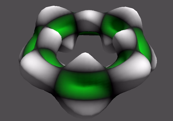
	PatternSample pattern_sample = sample_pattern(UV + animation_speed * TIME);

This produces a simple scrolling animation, causing the pattern to slide across the plane and loop around the torus.

In the next tutorial we will introduce fractal patterns. It will be released in the future.