Animating Octaves
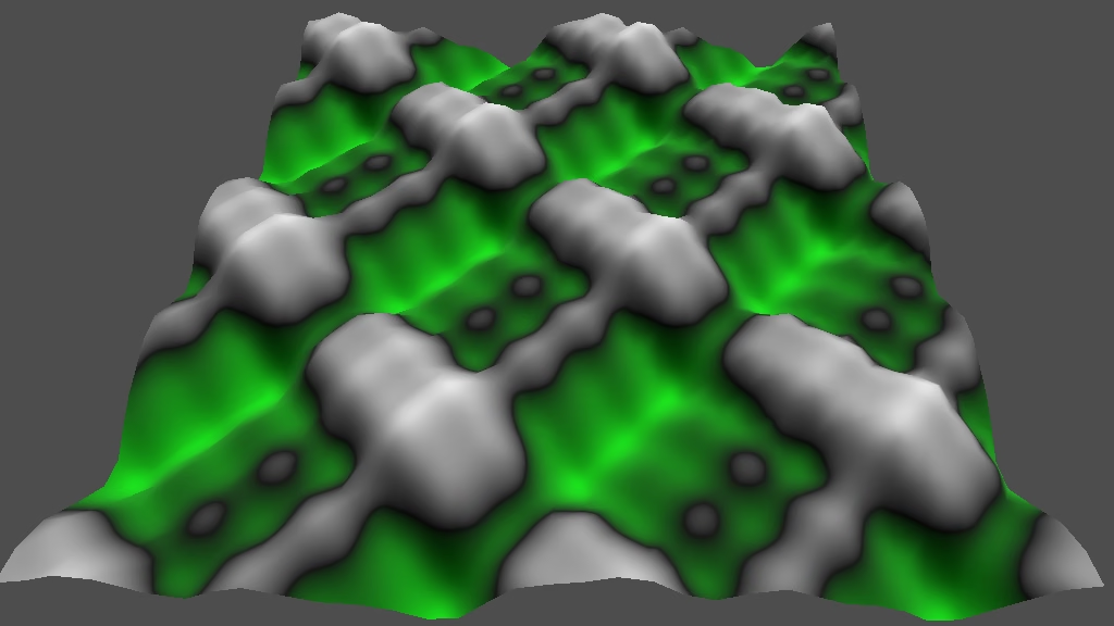
This is the sixth Godot tutorial in a series that covers the creation of procedural patterns on the GPU with shaders, using the Godot Engine, version 4.7. It follows Shader Library and adds support for per-octave animation to our fractals.
Animation Settings
Last time we introduced a shader library for the generation of fractal patterns. We used it for both the fractal sine waves and the hash patterns. However, these patterns are static. We do already animate the sine waves, by simply adding a time offset to the UV coordinates that we use to generate the fractal. So we only make the whole pattern slide uniformly, which is rather limiting. So let's add support for varying animation per octave, using the same fractal approach that we use for the pattern itself.
What we'll do is introduce a base_animation speed for the fractal, next to base_frequency, which gets applied to the first octave. We also include a temporal_lacunarity, which matches the regular lacunary used to scale the octaves. It is used to scale the time offset for successive octaves and is thus a measure of how the fractal fills time instead of space.
Previously we created the library first and added documentation as the lasts step. This time we do it the other way around and start with the documentation. So add documentation for the two new fractal settings to fractal_pattern_setings.gdshaderinc
. First include them in the settings list, placing them between persistence and adaptive_fractal_scale.
/*
Declares the FractalPatternSettings struct used by fractal_pattern.gdshaderinc.

The following settings are supported:
- base_frequency: Frequency of first octave (default 1.0 for all components).
- octaves: The amount of octaves (default 1).
- lacunarity: Frequency multiplier for successive octaves (default 2.0).
- persistence: Amplitude multiplier for successive octaves (default 0.5).
- base_animation: Animation speed for first octave (default 1.0).
- temporal_lacunarity: Animation multiplier for succesive octaves (default 2.0).
- adaptive_fractal_scale: How to scale the total amplitude (default false):
  - true: Based on actual octaves.
  - false: Based on infinite octaves.
We make the type of these settings configurable by defining PATTERN_ANIMATION_TYPE, just like PATTERN_FREQUENCY_TYPE.
/*
…
Define PATTERN_FREQUENCY_TYPE to set the type of base_frequency.
The default is float. Other options are float2, float3, float4.

Define PATTERN_ANIMATION_TYPE to set the type of
base_animation and temporal_lacunarity.
The default is float. Other options are float2, float3, float4.
It must either be float or match the frequency type.
For example, float for a uniform animation and vec2 for separate 2D frequencies.
Because animation is not always desired let's also use USE_FRACTAL_PATTERN_ANIMATION_SETTINGS to control whether animation uniform variables are included in the standard fractal pattern settings.
/*
…
Define USE_STANDARD_FRACTAL_PATTERN_SETTINGS to declare:
- Uniform variables for the default fractal pattern settings.
  Define USE_FRACTAL_PATTERN_ANIMATION_SETTINGS to also declare:
  - Uniform variables for fractal pattern animation.
- The standard_fractal_pattern_settings function to grab these settings.
Otherwise the default_fractal_pattern_settings function is declared.
Make sure that the default animation type is float.
#ifndef PATTERN_FREQUENCY_TYPE
#define PATTERN_FREQUENCY_TYPE float
#endif

#ifndef PATTERN_ANIMATION_TYPE
#define PATTERN_ANIMATION_TYPE float
#endif
Include the settings as fields in FractalPatternSettings.
struct FractalPatternSettings {
	PATTERN_FREQUENCY_TYPE base_frequency;
	int octaves;
	float lacunarity;
	float persistence;
	PATTERN_ANIMATION_TYPE base_animation;
	PATTERN_ANIMATION_TYPE temporal_lacunarity;
	bool adaptive_fractal_scale;
};
Set them to default values in default_fractal_pattern_settings().
FractalPatternSettings default_fractal_pattern_settings() {
	FractalPatternSettings settings = FractalPatternSettings(
			PATTERN_FREQUENCY_TYPE(1.0),
			1,
			2.0,
			0.5,
			PATTERN_ANIMATION_TYPE(1.0),
			PATTERN_ANIMATION_TYPE(2.0),
			false
	);
	return settings;
}
Optionally include uniform variables for them, if desired.
uniform float persistence : hint_range(0.0, 0.95, 0.05) = 0.5;
#ifdef USE_FRACTAL_PATTERN_ANIMATION_SETTINGS
uniform PATTERN_ANIMATION_TYPE base_animation = PATTERN_ANIMATION_TYPE(1.0);
uniform PATTERN_ANIMATION_TYPE temporal_lacunarity = PATTERN_ANIMATION_TYPE(2.0);
#endif
uniform bool adaptive_fractal_scale = false;
And use these variables in standard_fractal_pattern_settings() if they are declared, otherwise fall back to their default values.
FractalPatternSettings standard_fractal_pattern_settings() {
	return FractalPatternSettings(
			base_frequency,
			octaves,
			lacunarity,
			persistence,
#ifdef USE_FRACTAL_PATTERN_ANIMATION_SETTINGS
			base_animation,
			temporal_lacunarity,
#else
			PATTERN_ANIMATION_TYPE(1.0),
			PATTERN_ANIMATION_TYPE(2.0),
#endif
			adaptive_fractal_scale
	);
}
Fractal Animation
To actually use these new settings we move on to fractal_pattern.gdshaderinc
. We again begin with the documentation. First, sample_fractal_pattern() gets an extra float parameter for the time used for animation. We won't directly use TIME so the calling code can use whatever it wants to animate the fractal.
/*
Declares the sample_fractal_pattern function and whatever else it needs.
Its parameters are:
- FractalPatternSettings for the fractal settings.
- SAMPLE_PATTERN_COORDINATES_TYPE for the sample coordinates.
- float for the time used for animation.
The sample pattern function also gets an extra parameter for the octave's animation offset, which is the time value passed to the fractal function, adjusted based on the temporal lacunarity.
/*
…
Define SAMPLE_PATTERN_FUNCTION to set the function for sampling an octave.
Only define the function name, without parameter list.
The matching function declaration must have three parameters:
- int for the octave's index.
- PATTERN_FREQUENCY_TYPE for the octave's sample frequency.
- SAMPLE_PATTERN_COORDINATES_TYPE for the sample coordinates.
- PATTERN_ANIMATION_TYPE for the octave's animation offset.
Frequency must either be float or match the coordinates type.
For example, float for a uniform frequency and vec2 for 2D sample coordinates.
Add the new parameter to dummy_sample_pattern().
PatternSample dummy_sample_pattern(
		int octave,
		PATTERN_FREQUENCY_TYPE frequency,
		SAMPLE_PATTERN_COORDINATES_TYPE coordinates,
		PATTERN_ANIMATION_TYPE animation_offset
) {
	return zero_pattern_sample();
}
Then adjust sample_fractal_pattern() so it scales the given time with the base animation factor. Then pass that animation offset to the sample pattern function inside the loop, followed by scaling it with the temporal lacunarity. I pulled the sample call out of the summation code line and put it in a sample variable for clarity.
PatternSample sample_fractal_pattern(
		FractalPatternSettings settings,
		SAMPLE_PATTERN_COORDINATES_TYPE coordinates,
		float time
) {
	PatternSample sum = zero_pattern_sample();
	PATTERN_FREQUENCY_TYPE frequency = settings.base_frequency;
	PATTERN_ANIMATION_TYPE animation_offset = settings.base_animation * time;
	float amplitude = 1.0;
	for (int i = 0; i < settings.octaves; i++) {
		PatternSample sample = SAMPLE_PATTERN_FUNCTION(
				i, frequency, coordinates, animation_offset
		);
		sum = add(sum, multiply(sample, amplitude));
		frequency *= settings.lacunarity;
		animation_offset *= settings.temporal_lacunarity;
		amplitude *= settings.persistence;
	}
	return normalize_fractal_sample(settings, sum);
}
We now have to adjust our shaders to match the changed function signatures. First hashing.gdshader
. Add a float parameter for the octave's time offset to sample_hash(). We can simply call it time, knowing that it is specific to the octave.
PatternSample sample_hash(int octave, float frequency, vec2 uv, float time) { … }Also add TIME as an argument to sample_factal_pattern().
void fragment() {
	ALBEDO = sample_fractal_pattern(
			standard_fractal_pattern_settings(),
			UV - 0.5,
			TIME
	).v;
}
Second sine_waves.gdshader
, again adding the time parameter.
PatternSample sample_pattern(int octave, vec2 frequency, vec2 uv, float time) { … }And adding TIME as an argument inside both vertex() and fragment().
	PatternSample pattern_sample = sample_fractal_pattern(
			standard_fractal_pattern_settings(),
			UV + animation_speed * TIME,
			TIME
	);
This fixes our shaders and they still produce the same results, because we're ignoring the per-octave time. So all the code that we added up to this point gets optimized away by the shader compiler.
Sine Waves Animation
Now we can upgrade the existing animation of sine_waves.gdshader
to the more flexible fractal approach. Replace the animation_speed uniform variable with the standard fractal animation settings, using vec2 for the pattern animation type to keep supporting independent animation for U and V.
//uniform vec2 animation_speed = vec2(0.0);
uniform vec2 bumpiness = vec2(1.0);
uniform float displacement : hint_range(-1.0, 1.0) = 0.2;

#define PATTERN_FREQUENCY_TYPE vec2
#define PATTERN_ANIMATION_TYPE vec2
#define USE_STANDARD_FRACTAL_PATTERN_SETTINGS
#define USE_FRACTAL_PATTERN_ANIMATION_SETTINGS
#include "res://shader_library/fractal_pattern_settings.gdshaderinc"
Change the type of the time paramater of sample_pattern() to match. Then apply the per-octave animation by adding the 2D time offset to the given UV coordinates, before scaling them with the frequency.
PatternSample sample_pattern(int octave, vec2 frequency, vec2 uv, vec2 time) {
	vec2 f = frequency * TAU;
	vec2 t = f * (uv + time);
	…
}
That takes care of all animations, so we have to remove the time offset that we add to UV in vertex() and fragment().
	PatternSample pattern_sample = sample_fractal_pattern(
			standard_fractal_pattern_settings(),
			UV,
			TIME
	);
Let's see what we can do with these animation settings. For simplicity we'll use sine_waves_plane.tscn
and limit ourselves to only a single dimension, using the U function. Set base frequency to 2 with only two octaves, and a base animation of 0.25 so it doesn't move too fast. If we look at temporal lacunary 1 first we get the same uniform sliding animation that we had before.
If we set temporal lacunarity to 2 then the second octave will move twice as fast as the first octave. This makes the smaller waves slide along the larger waves, moving ahead of them.
We can also flip the temporal relationship around by setting temporal lacunarity to 0.5, which makes the smaller waves fall behind the larger waves.
We could go a step further and freeze the second octave by reducing temporal lacunarity to zero.
And we can even make it negative. By using −1 successive octaves move in opposite directions, which produces a very different animation.
Going further to −2 makes this more pronounced.
Now that we have a decent understanding of how the animation works we can move on to 2D patterns. For example, the UV product function, with 3 octaves, base animation (0.1, 0.2), and temporal lacunarty (1.5, 1.25).
And for a final example let's go to sine_waves_torus.tscn
and use the UV average function, base frequency (3, 2), 3 octaves, base animation (0.2, 0.1), and temporal lacunarity (0.5, 1.5).
Hash Animation
To also support animation for our fractal hash in hashing.tscn
include the standard fractal animation settings in hashing.gdshader
. In this case we use the default one-dimensional time type.
#define USE_STANDARD_FRACTAL_PATTERN_SETTINGS
#define USE_FRACTAL_PATTERN_ANIMATION_SETTINGS
We can animate the pattern in the same way as the waves by adding the time offset to the UV coordinates before scaling them with the frequency in sample_hash().
vec2 coordinates = floor(frequency * (uv + time));To make the animation easiest to see set the visualization to grayscale. Use the default fractal settings, with base frequency 8, 2 octaves, and base animation 0.25. This gives two overlapping octaves that slide diagonally.
A sliding animation isn't the most interesting nor the most useful way to animate our hash pattern. What we'll do instead is incorporate the floored time into the hash calculation. That will make the pattern change in unpredictable ways at regular intervals.
	vec2 coordinates = floor(frequency * uv);
	Hasher h = hasher(hash_seed + uint(octave));
	h = hasher(h, coordinates.x);
	h = hasher(h, coordinates.y);
	h = hasher(h, floor(time));
uint hash = hash(h);Staggered Hash Animation
By incorporating the time uniformly into the hash we're effectively treating it as a third spatial dimension and sliding a 2D slice through it. Thus all hashes of an octave change at the same time. Because our temporal lacunarity is set to 2 the second octave changes twice as fast as the first one. This produces a temporal pattern of a big change, when both octaves change together, followed by a small change, when only the second octave changes, followed by another big change, and so on. The result is an obvious pulsing temporal pattern.
We can make the temporal pulsing less obvious by no longer changing all hashes of an octave at the same time. We do this by introducing temporal offsets based on the hash coordinates, thereby distorting the temporal dimension. We can do this because we're not actually moving through 3D space, we're changing independent hash blocks. Changing them at different times won't warp the pattern. We could even animate individual blocks at different speeds.
To get the best results we must ensure that the temporal offset produces a uniform pattern without temporal directionality. The simplest way to do this is by offsetting the time for every other hash block by 0.5, thus producing a checkered grid. We can make such a grid by adding the hash coordinates together, halving them, and taking the fractional part. That gives a checkered pattern with blocks that are either 0.0 or 0.5. To demonstrate that this works let's temporarily override the sample value with that offset.
	s.v = vec3(fract((coordinates.x + coordinates.y) * 0.5));
	return s;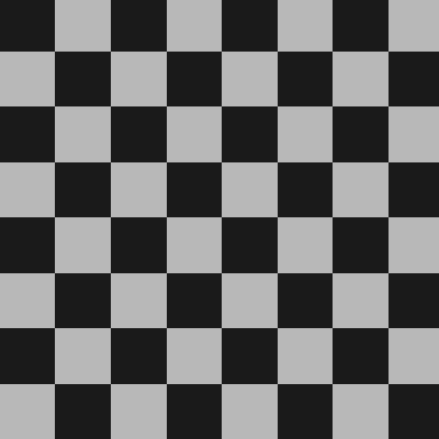
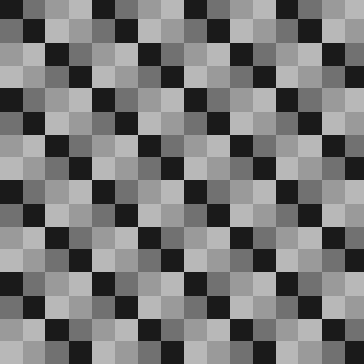
To use this as an extra time offset add it to the time before flooring it. Let's also make this staggered animation optional by introducing a uniform variable toggle for it, so it's easier to compare animation with and without it.
uniform int visualization : hint_enum("Grayscale", "RG", "RGB") = 0;
uniform bool staggered_animation = true;

…

PatternSample sample_hash(int octave, float frequency, vec2 uv, float time) {
	…
	if (staggered_animation) {
		time += fract((coordinates.x + coordinates.y) * 0.5);
	}
	h = hasher(h, floor(time));
	…
	//s.v = vec3(fract((coordinates.x + coordinates.y) * 0.5));
	return s;
}The animation speed is still the same for each individual hash block, but because half the pattern has the 0.5 temporal offset the observed total pattern appears to animate twice as fast as before. But because only half the pattern changes at any given time the temporal pulsing has also become less obvious.
We could use more than two time offsets, for example by scaling the summed coordinates by 0.25 instead of 0.5. That produces a four-step gradient pattern.
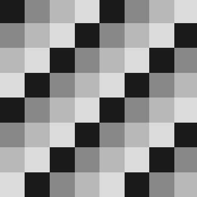
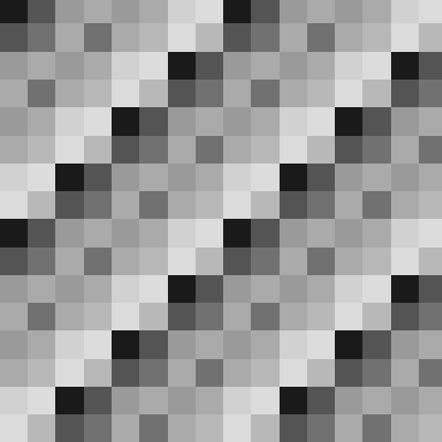
However, such patterns aren't symmetrical and exhibit diagonal temporal movement. So it's best to stick with the checkered grid.
To wrap up here's an animated RGB hash with three octaves.
The next tutorial is Value Noise.