Tiling Noise
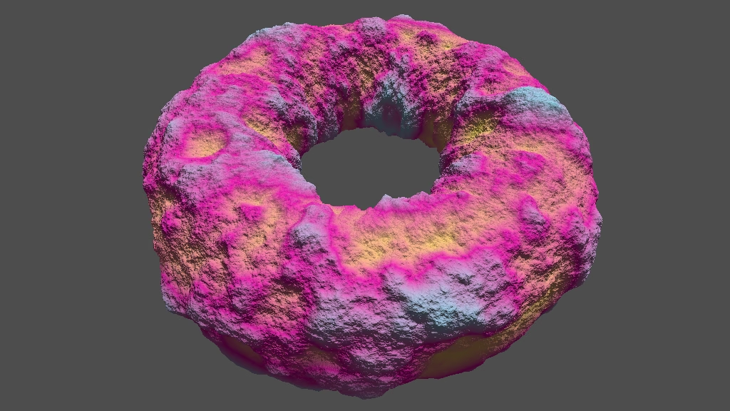
This is the ninth Godot tutorial in a series that covers the creation of procedural patterns on the GPU with shaders, using the Godot Engine, version 4.7. It follows Value Noise Derivatives and adds tiling to it.
Value Noise on Torus
Up to this point we have only considered value noise applied to a plane. Let's also take a look at how it gets applied to a torus. Create a value_noise_torus.tscn
scene like sine_waves_torus.tscn
but with a material matching the one used in value_noise_plane.tscn
. Leave the displacement at its default 0.2 otherwise the torus will get too thick.
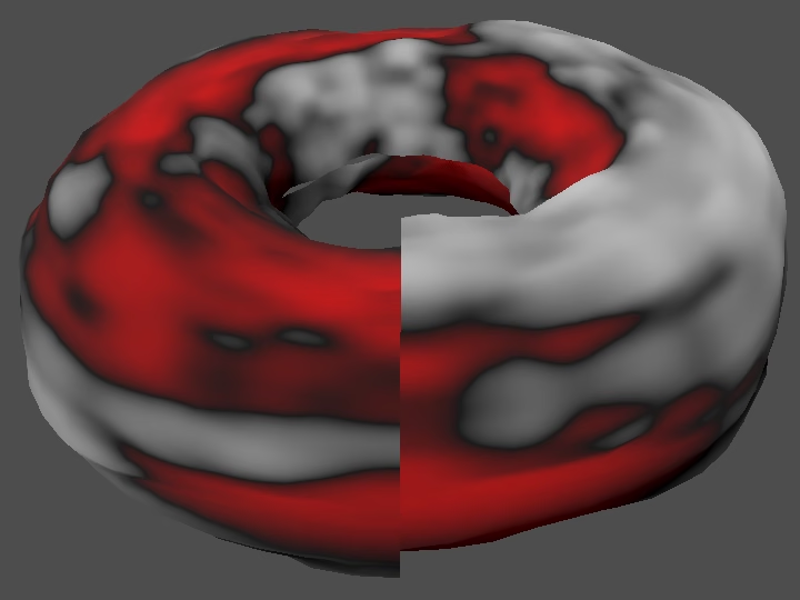
The torus has two obvious seams where UV coordinates 0 and 1 meet. We'll deal with that later. Let's first upgrade the bumpiness and frequency types to vec2 in value_noise.gdshader
so we can better tune them for the torus, like we did for the sine waves in the past.
uniform vec2 bumpiness = vec2(1.0);
uniform float displacement : hint_range(-1.0, 1.0) = 0.2;
uniform bool vertex_displacement = true;

#define PATTERN_FREQUENCY_TYPE vec2
#define USE_STANDARD_FRACTAL_PATTERN_SETTINGS
Adjust sample_value_noise() to work with the new frequency type.
PatternSample sample_value_noise(
		int octave,
		vec2 frequency,
		vec2 uv,
		float time
) {
	…
	s.dx *= frequency.x;
	s.dy *= frequency.y;
	return s;
}
Now we have to reconfigure the plane scene, duplicating the old values for both components of the bumpiness and frequency. For the torus we again use (0.212, 0.637) for the bumpiness and let's set its base frequency to (6,4).
Testing UV Range
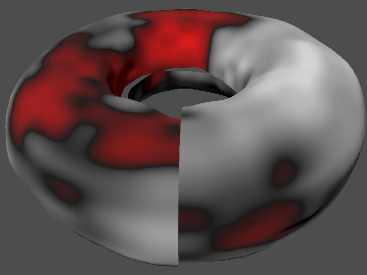
To make the pattern seamlessly wrap around the torus we'll have to tile it, so that it repeats itself for coordinates below 0 and above 1. To try this out we'll temporarily switch back to the plane. At the moment we've set UV coordinates to go from −0.5 to 0.5. We set the plane's base frequency to 4 with only a single octave and see what we get.
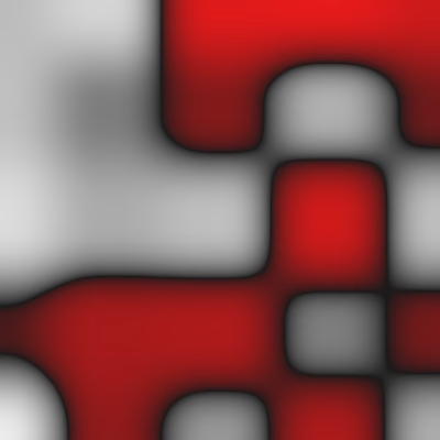
To test tiling we'll change the UV to go from −1 to 2 instead. Introduce a sample_noise() function that we use it both vertex() and fragment() so we only have to adjust the UV range in one place from now on.
PatternSample sample_noise(vec2 uv) {
	return sample_fractal_pattern(
			standard_fractal_pattern_settings(),
			uv * 3.0 - 1.0,
			TIME
	);
}

void vertex() {
	if (vertex_displacement) {
		PatternSample pattern_sample = sample_noise(UV);
		VERTEX += NORMAL * (pattern_sample.v * displacement);
	}
}

void fragment() {
	PatternSample pattern_sample = sample_noise(UV);
	ALBEDO = colorize(pattern_sample.v);
	…
}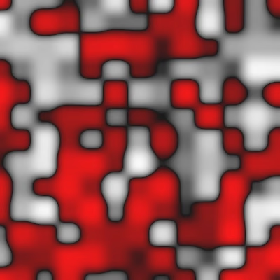
Because the usual UV range goes from 0 to 1 our goal is to tile the pattern in that UV range. That's the central tile in the middle of our plane right now. This tile is surrounded by eight tiles that are currently showing different patterns. When we're done all nine tiles in the 3×3 region should show the exact same pattern, without seams between them.
Tiling Lattice Coordinates
If we were using the hash noise pattern we could suffice with taking the fractional part of the UV coordinates and the pattern would tile perfectly. However, seams are part of the pattern so that provides no benefit. But value noise blends between adjacent lattice points, so we also have to blend across tile boundaries to eliminate the seams. This means that the lattice blocks at the tile boundaries must wrap their lattice points to match the opposite side of the tile.
For example, with frequency 4 the lattice coordinate sequence in one dimension is 0, 1, 2, 3, 4 for a single tile. Broken up into lattice blocks we get the lattice point pair sequence (0,1), (1,2), (2,3), (3,4). When tiling the end must wrap back to the beginning, so the coordinate sequence becomes 0, 1, 2, 3, 0 and the blocks become (0,1), (1,2), (2,3), (3,0).
Because we'll need to modify lattice coordinates we introduce a lattice01() function that sample_value_noise() will use to get the first and second lattice coordinates for the lattice block in a single dimension. It takes the original lattice coordinate and returns it and the next one, which we'll locally name l0 and l1. We return them packed in a vec2. To perform tiling we'll also need to know the frequency.
vec2 lattice01(float lattice_coordinate, float frequency) {
	float l0 = lattice_coordinate;
	float l1 = l0 + 1.0;
	return vec2(l0, l1);
}
Adapt sample_value_noise() to use this function.
	vec2 fractional_coordinates = sample_coordinates - lattice_coordinates;

	vec2 uLattice = lattice01(lattice_coordinates.x, frequency.x);
	vec2 vLattice = lattice01(lattice_coordinates.y, frequency.y);

	Hasher h = hasher(hash_seed + uint(octave));
	Hasher h0 = hasher(h, uLattice.x);
	Hasher h1 = hasher(h, uLattice.y);
	Hasher h00 = hasher(h0, vLattice.x);
	Hasher h10 = hasher(h1, vLattice.x);
	Hasher h01 = hasher(h0, vLattice.y);
	Hasher h11 = hasher(h1, vLattice.y);
Now we can start adjusting the coordinates in lattice01() to repeat the pattern in the 3×3 block region that we're observing. Let's first consider negative coordinates. To make these match the central tile we have to modify them so they become positive, which we do by adding the frequency to l0.
	float l0 = lattice_coordinate;
	if (l0 < 0.0) {
		l0 += frequency;
	}
	float l1 = l0 + 1.0;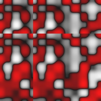
This produces partial tiling on the negative side, along with a seam. To get rid of the seam we have to shift l1 to the left side if it's on the right side of the tile, so when it ends up equal to or larger than the frequency.
	float l1 = l0 + 1.0;
	if (l1 >= frequency) {
		l1 -= frequency;
	}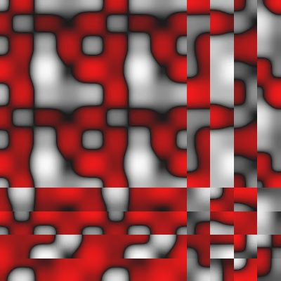
This seamlessly tiles on the negative side, although it turns the tiles on the positive side into a mess. To fix those tiles we have to make the same adjustment to l0 that we made to l1, if it didn't start out negative.
	float l0 = lattice_coordinate;
	if (l0 < 0.0) {
		l0 += frequency;
	}
	else if (l0 >= frequency) {
		l0 -= frequency;
	}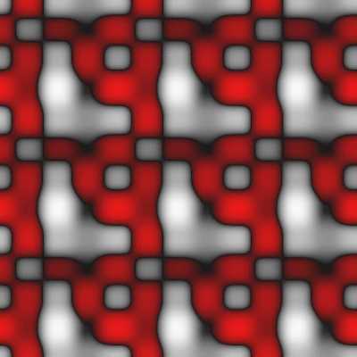
Now we get perfect seamless tiling for the entire 3×3 region. However, it fails for larger regions, which becomes visible if we expand the visible region to 5×5.
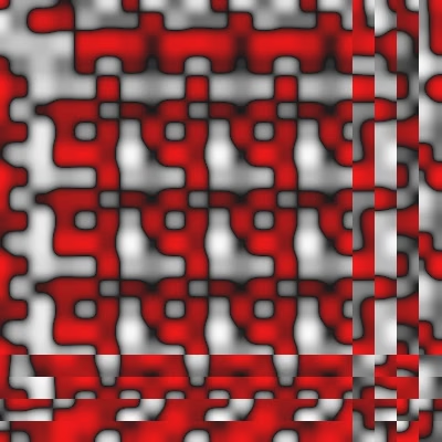
This limitation is acceptable, because the goal is to seamlessly match UV coordinates 0 and 1. Our current cheap and simple approach supports this. It even works up to −1 and 2, so we can go at most one unit outside the 0–1 range. That allows for some wiggle room, for example for sliding animations, which we'll add later.
However, there is an additional limitation: the frequency must be a whole number so lattice points align with the tile edges. Otherwise the pattern will no longer tile.
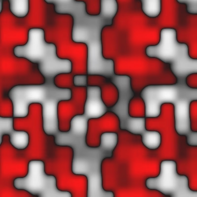
Finally, tiling works with animation, but only when even frequencies are used. This is because we use staggered animation. If the frequency is odd then lattice blocks on opposite sides of the tile will use different time offsets for their matching lattice points.
Optional Tiling
Tiling usually isn't needed, so let's add a toggle option for it and disable it by default. It is also possible to add support for optional tiling per dimension, but we keep it simple and make it all-or-nothing deal. Let's also add some code documentation that explains the tiling ands its requirements, using a multiline comment in between /* */. By adding a second * to the opening statement the Godot editor's inspector will also display it as a tooltip for the shader parameter.
uniform uint hash_seed = 0u;
/**
Seamlessly tile pattern for UV from 0 to 1.
Tiling works for UV in between -1 and 2.
Requires integer frequencies for all octaves.
Requires even frequencies for animation.
*/
uniform bool tiling = false;
If tiling is disabled then we revert to the original approach in lattice01().
vec2 lattice01(float lattice_coordinate, float frequency) {
	if (!tiling) {
		return vec2(lattice_coordinate, lattice_coordinate + 1.0);
	}
	else {
		float l0 = lattice_coordinate;
		if (l0 < 0.0) {
			l0 += frequency;
		}
		else if (l0 >= frequency) {
			l0 -= frequency;
		}
		float l1 = l0 + 1.0;
		if (l1 >= frequency) {
			l1 -= frequency;
		}
		return vec2(l0, l1);
	}
}
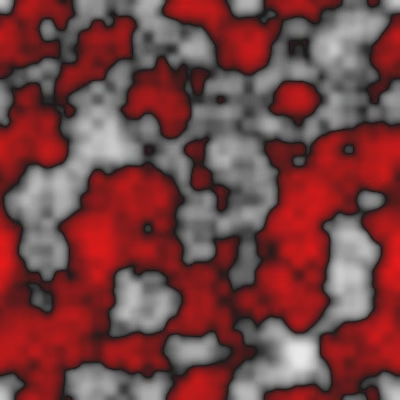
With testing done we reduce the UV range back to a single unit. We won't subtract the old 0.5 offset anymore.
PatternSample sample_noise(vec2 uv) {
	return sample_fractal_pattern(
			standard_fractal_pattern_settings(),
			uv,
			TIME
	);
}
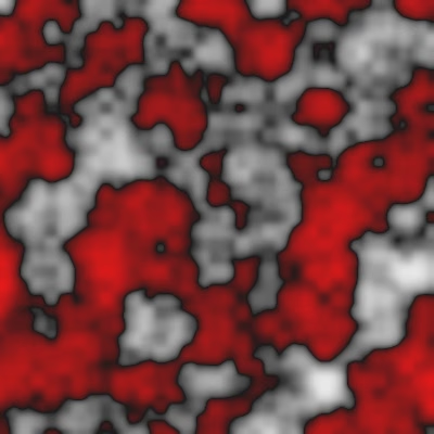
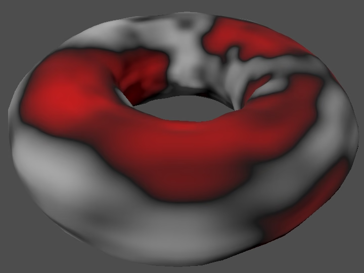
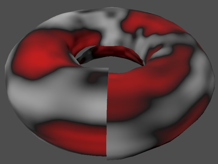
Now we can finally get a seamless value noise pattern wrapped around our torus. I increased the torus rings to 128 and its ring segments to 64 to make it smoother.
Animation
As stated earlier, tiling also works with animation as long as the frequencies of all octaves are even.
Let's wrap up by also adding support for sliding animation, which can make the animation of the torus look more interesting. Add a separate configuration option for a slide velocity.
uniform bool animation = true;
uniform vec2 slide_velocity = vec2(0.0, 0.0);
If animation is enabled use the slide velocity scaled by TIME to offset the UV coordinates in sample_noise().
PatternSample sample_noise(vec2 uv) {
	if (animation) {
		vec2 slide_offset = slide_velocity * TIME;
		uv += slide_offset;
	}
	return sample_fractal_pattern(
			standard_fractal_pattern_settings(),
			uv,
			TIME
	);
}
This will quickly break tiling, because we go outside the supported UV region. So we have to limit the offset to a single unit at most, by only adding its fractional part to the UV coordinates. This ensures that we always stay inside the valid region.
		vec2 slide_offset = slide_velocity * TIME;
		if (tiling) {
			slide_offset = fract(slide_offset);
		}
		uv += slide_offset;
We'll investigate an alternative value noise pattern in the future.