Value Noise Derivatives
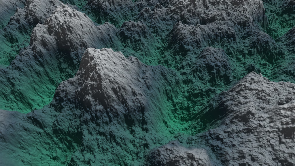
This is the eighth Godot tutorial in a series that covers the creation of procedural patterns on the GPU with shaders, using the Godot Engine, version 4.7. It follows Value Noise and adds the derivative functions for it.
Adjusting Normal Vectors
We calculate the derivatives for our sine wave function so we can generate correct surface normals for it. We didn't do this for hash noise because it doesn't produce a smooth continuous surface. Each isolated block of its pattern is constant and thus its derivatives are always zero. But value noise turns that into a smooth continuous pattern, so we could calculate its derivatives to produce a bumpy surface, just like for the sine waves.
We'll copy some code from sine_waves.gdshader
to value_noise.gdshader
. We begin with the fragment normal vectors only, leaving vertex displacement for later. Insert uniform float variables for the bumpiness and displacement and use them with the pattern's derivatives to generate the view-space normal vector in fragment().
uniform vec3 color_max : source_color = vec3(1.0);
uniform float bumpiness = 1.0;
uniform float displacement : hint_range(-1.0, 1.0) = 0.2;
…

void fragment() {
	PatternSample pattern_sample = …
	ALBEDO = colorize(pattern_sample.v);

	vec2 d =
			vec2(pattern_sample.dx, pattern_sample.dy) *
			displacement * bumpiness;
	NORMAL = cross(
			TANGENT + NORMAL * d.x,
			BINORMAL - NORMAL * d.y
	);
}
Set the bumpiness to 0.5 so the normal vectors will be properly aligned for our plane's size, like we did for the sine waves plane.
Blending Pattern Samples
We still get the same normals because the derivatives of the final pattern sample are zero as we don't set them. We have to include the derivatives when calculating value noise, which means when blending the hash values.
We make the pattern smooth by blending between the four lattice point samples of each block, using mix(). When doing so we'll also have to mix the derivatives along with the sample values. To make this easier let's add a blend() function to pattern_sample.gdshadering
that reproduces mix(), with PatternSample parameters replacing the float parameters. Initially it only mixes the sample value, still leaving the derivatives at zero.
PatternSample blend(PatternSample a, PatternSample b, PatternSample t) {
	PatternSample sample = zero_pattern_sample();
	sample.v = mix(a.v, b.v, t.v);
	return sample;
}
To use this function in value_noise.gdshader
we have to provide it with the needed pattern samples, of which there are four. Let's add a convenient value_sample() function that calls animated_hash_to_float() for a given hasher and time, then puts that in a pattern sample.
PatternSample value_sample(Hasher h, float time) {
	PatternSample sample = zero_pattern_sample();
	sample.v = animated_hash_to_float(h, time);
	return sample;
}
Now we can upgrade our four lattice values to pattern samples in sample_value_noise(). We have to also introduce pattern samples for the interpolators used for blending. Then we can replace mix() with blend().
	PatternSample v00 = value_sample(h00, timeA);
	PatternSample v10 = value_sample(h10, timeB);
	PatternSample v01 = value_sample(h01, timeB);
	PatternSample v11 = value_sample(h11, timeA);
	//PatternSample s = zero_pattern_sample();
	vec2 t = smoothstep(0.0, 1.0, fractional_coordinates);
	PatternSample tx = zero_pattern_sample();
	tx.v = t.x;
	PatternSample ty = zero_pattern_sample();
	ty.v = t.y;
	PatternSample s = blend(
			blend(v00, v10, tx),
			blend(v01, v11, tx),
			ty
	);
Also, just like for sine waves we have to scale the derivatives with the frequency at the end.
	s.dx *= frequency;
	s.dy *= frequency;
	return s;
Linear Blending
We can now start calculating the derivatives. To begin simple let's first revert the noise back to linear mixing, by removing the smoothing of the interpolators.
	//vec2 t = smoothstep(0.0, 1.0, fractional_coordinates);
	vec2 t = fractional_coordinates;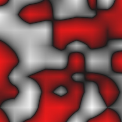
Now the derivatives of the interpolators are trivial: they're 1 for their respective dimension.
	PatternSample tx = zero_pattern_sample();
	tx.v = t.x;
	tx.dx = 1.0;
	PatternSample ty = zero_pattern_sample();
	ty.v = t.y;
	ty.dy = 1.0;
To calculate the derivatives of mix() we have to compute it ourselves, for which we'll use its simplest mathematical form:
pattern_sample.gdshader
already contains the add() function for two patterns samples, but now we also need a subtract() function.
PatternSample subtract(PatternSample a, PatternSample b) {
	return PatternSample(
			a.v - b.v,
			a.dx - b.dx,
			a.dy - b.dy,
			a.dz - b.dz
	);
}
We also have to add a multiply() function for two pattern samples. To get the correct derivatives for that we need to apply the product rule:
In general, if we have a function then its derivative function is .
Suppose that we also have a second function with its derivative function .
If we have a third function then what is ?
We know , but it gets scaled by . Conversely, we know but it gets scaled by . The final derivative is exactly that, added together:
PatternSample multiply(PatternSample a, PatternSample b) {
	return PatternSample(
			a.v * b.v,
			b.v * a.dx + a.v * b.dx,
			b.v * a.dy + a.v * b.dy,
			b.v * a.dz + a.v * b.dz
	);
}
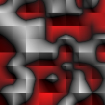
Now we can use our own math functions to replace mix() in blend(), also taking care of the derivatives.
PatternSample blend(PatternSample a, PatternSample b, PatternSample t) {
	return add(a, multiply(subtract(b, a), t));
}
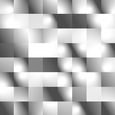
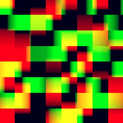
To clearly see the derivatives of the pattern I also temporarily used them directly for RG colors, so only positive derivatives are visible:
Smooth Blending
We want a smooth pattern so the next step is to introduce a replacment for smoothstep() that works with derivatives. We add such a function to pattern_sample.gdshaderinc
, naming it smooth01() to indicate that it works for values from 0 to 1. Initially we only smooth the value and leave the derivatives at zero.
PatternSample smooth01(PatternSample t) {
	return PatternSample(
		smoothstep(0.0, 1.0, t.v),
		0.0,
		0.0,
		0.0
	);
}
Use this function in sample_value_noise() in value_noise.gdshader
to smooth the interpolators.
	PatternSample tx = zero_pattern_sample();
	tx.v = t.x;
	tx.dx = 1.0;
	tx = smooth01(tx);
	PatternSample ty = zero_pattern_sample();
	ty.v = t.y;
	ty.dy = 1.0;
	ty = smooth01(ty);
To get the correct derivatives we need to find the derivative function of smoothstep(). We already know the function itself:
Its derivative function is:
We can rewrite this to a simpler form with fewer multiplications:
Use that function to calculate the derivatives in smooth01()in pattern_sample.gdshaderinc
.
PatternSample smooth01(PatternSample t) {
	PATTERN_SAMPLE_VALUE_TYPE d = (6.0 - 6.0 * t.v) * t.v;
	return PatternSample(
		smoothstep(0.0, 1.0, t.v),
		d,
		d,
		d
	);
}
We also have to incorporate the derivatives of the original sample into the final derivatives. For that we have to apply the chain rule:
In general, if we have a function then its derivative function is .
Suppose that we also have a second function with its derivative function .
If we have a third function then what is ?
We know , but what gets passed to it is first passed through . Thus gets scaled by :
	return PatternSample(
		smoothstep(0.0, 1.0, t.v),
		d * t.dx,
		d * t.dy,
		d * t.dz
	);
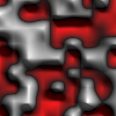
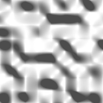
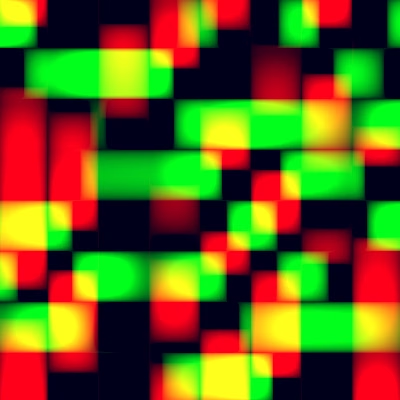
In this case we use the cain rule to select which derivative is set, because the interpolator derivatives are either 0 or 1. We use the same chain rule when scaling the derivatives by the octave's frequency, because the frequency application is a simple scaling function.
Smoother Blending
We now have a smooth pattern with correct normal vectors, but it doesn't look as smooth as we might have expected. There appear to be sharp creases along lattice edges. To figure out why this is the case we go back to visualizing our mix functions:
That the linear option has sharp edges is immediately clear. But to find the cause of the sharp creases of the smooth option we have to go a step further and look at its second derivative function. This is the derivative of the derivative, so the rate of change of the rate of change, which is its acceleration:
The below graph shows the first and second derivative functions matching the previous graph. We only care about the shape of the curves and not their exact scales, so they're normalized to an amplitude of 1.
Both derivatives are continuous, but the second derivative is not smooth. In this case the result still appears fine, because this test case is symmetrical. What if we made it asymmetrical, by changing the lattice value sequence from 0–1–0 to 0–1–0.5?
Now we get a crease at the lattice edge. The first derivative is not longer smooth, because the second derivative is no longer continuous. Let's also consider 0–0.5–1, which at first glance might appear smoother:
This produces a staircase pattern with an even more pronounced crease.
The problem is that the second derivative is nonzero at the lattice edges. To get rid of the creases we have to ensure that both the first and second derivative functions are zero at the lattice edges. We can use the following function for that, which is a more extreme version of smoothstep, hence often known as smootherstep:
This function can also be rewritten to minimize multiplications:
Here is its first derivative function, in regular and mimimized form:
And here is its second derivative function, also in both forms:
Let's first show it for the original symmetrical 0–1-0 case:
That looks good. Here's the asymmetrical 0–1–0.5 case:
The second derivative indeed remains continuous. And here is the 0–0.5–1 staircase:
This works, so we add a smoother01() function to pattern_sample.gdshaderinc
.
PatternSample smoother01(PatternSample t) {
	PATTERN_SAMPLE_VALUE_TYPE d =
			t.v * t.v * (t.v * (30.0 * t.v - 60.0) + 30.0);
	return PatternSample(
		t.v * t.v * t.v * (t.v * (6.0 * t.v - 15.0) + 10.0),
		d * t.dx,
		d * t.dy,
		d * t.dz
	);
}
Switch to it in sample_value_noise() in value_noise.gdshader
.
	PatternSample tx = zero_pattern_sample();
	tx.v = t.x;
	tx.dx = 1.0;
	tx = smoother01(tx);
	PatternSample ty = zero_pattern_sample();
	ty.v = t.y;
	ty.dy = 1.0;
	ty = smoother01(ty);
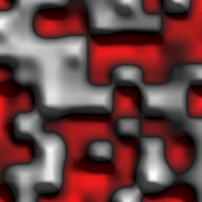
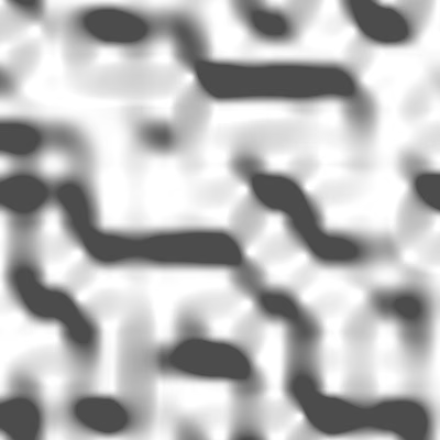
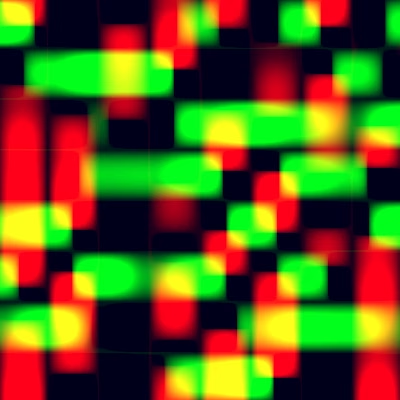
Smoother blending gets rid of the creases. It doesn't get rid of the staircases, because that's an inherent feature of smooth blending.
Configurable Smoothness
Smoother blending is only really needed when derivatives are used to adjust normal vectors. If the pattern is only used for coloring then smooth blending suffices. Linear blending might also be desired as an artistic choice. So let's add a variant smooth01() function to pattern_sample.gdshaderinc
that has an extra int parameter for a smoothness type. Smoothness 1 is linear, which is the original sample unmodified. Smoothness 2 is smooth, while smoothness 3 is smoother.
PatternSample smooth01(PatternSample t, int smoothness_type) {
	switch(smoothness_type) {
		case 1:
			return t;
		case 2:
			return smooth01(t);
		case 3:
			return smoother01(t);
	}
}
Let's also include a fourth option for a harsh binary transition, stepping from 0 to 1 at the halfway point. We use that as the default option, so for smoothness 0 or any other value.
		case 3:
			return smoother01(t);
		default:
			PatternSample s = zero_pattern_sample();
			s.v = step(PATTERN_SAMPLE_VALUE_TYPE(0.5), t.v);
			return s;
Add a uniform int variable to value_noise.gdshader
to configure it, displayed as an enumeration with appropriate labels, set to smoother by default.
uniform int smoothness : hint_enum("Step", "Linear", "Smooth", "Smoother") = 3;
uniform float bumpiness = 1.0;
Then use the configurable smooth01() function in sample_value_noise().
	PatternSample tx = zero_pattern_sample();
	tx.v = t.x;
	tx.dx = 1.0;
	tx = smooth01(tx, smoothness);
	PatternSample ty = zero_pattern_sample();
	ty.v = t.y;
	ty.dy = 1.0;
	ty = smooth01(ty, smoothness);
Now we can easily change and compare the different smoothness options. The step option effectively eliminates blending and turns value noise into hash noise.
Vertex Displacement
We wrap up by adding vertex displacement like we did for the sine waves. Add a toggle option for it, enabled by default.
uniform float displacement : hint_range(-1.0, 1.0) = 0.2;
uniform bool vertex_displacement = true;
Then introduce the required vertex() function.
void vertex() {
	if (vertex_displacement) {
		PatternSample pattern_sample = sample_fractal_pattern(
				standard_fractal_pattern_settings(),
				UV - 0.5,
				TIME
		);
		VERTEX += NORMAL * (pattern_sample.v * displacement);
	}
}
I set the subdivide level of the plane to 63 to get smoother surfaces.
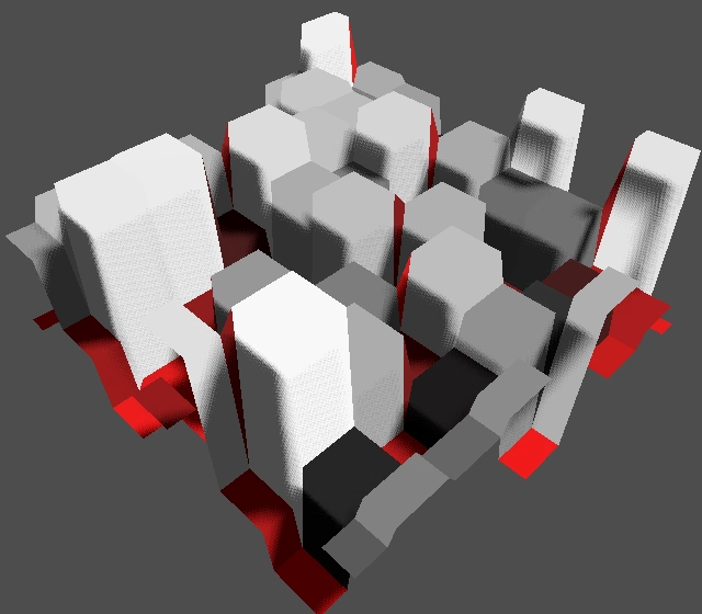
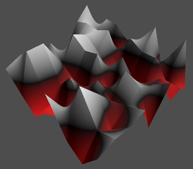
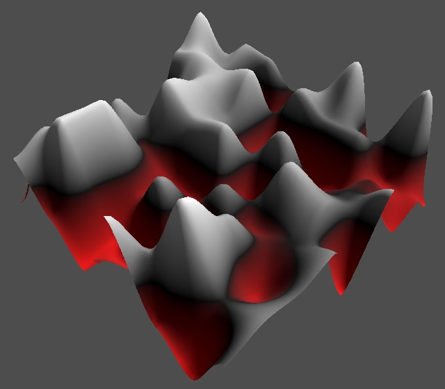
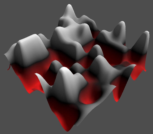
Finally, here is smoother value noise with displacement animated:
The next tutorial is Tiling Noise.