Fractal Waves
This is the third tutorial in a series that covers the creation of procedural patterns on the GPU with shaders, using the Godot Engine, version 4. It follows 2D Waves and expands it to create fractal patterns.
This tutorial uses Godot 4.6, the regular version, but you could also use the .NET version.
Multiple Layers of Waves
A fractal is something that displays self-similarity, meaning that it exhibits similar patters at different scales. When you zoom in on part of such a pattern you'll see the same pattern again, integrated into the larger pattern. These patterns occur naturally and can also be made mathematically.
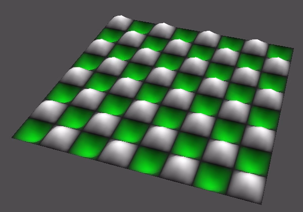
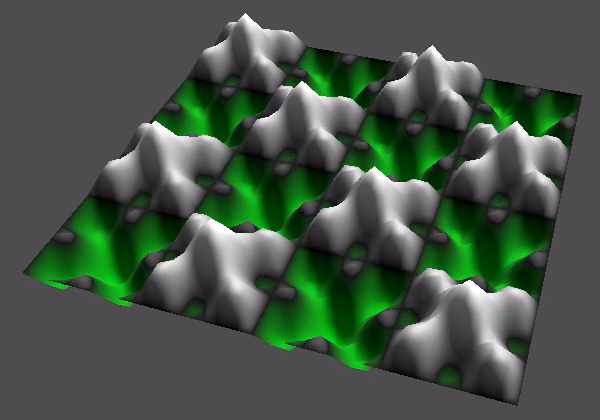
In our case we can turn the wave patterns into fractals by layering multiple of them on top of each other, each with different frequencies. For example, let's consider the UV Product pattern on the plane. Starting with uniform frequency 2, we can make it fractal-like by including a second layer of it, with its frequency doubled to 4. If we also halve the displacement of the second layer it looks like a half-sized version of the first layer.

To create the fractal we'll have to sample the pattern more than once. Let's add a sample_fractal_pattern() function to sine_waves.gdshader
that will take care of constructing the fractal and call it instead of sample_pattern() in vertex() and fragment(). Initially it just samples the pattern once.
PatternSample sample_fractal_pattern(vec2 uv) {
	return sample_pattern(uv);
}

void vertex() {
	PatternSample pattern_sample = sample_fractal_pattern(
			UV + animation_speed * TIME
	);
	…
}

void fragment() {
	PatternSample pattern_sample = sample_fractal_pattern(
			UV + animation_speed * TIME
	);
	…
}
Adding Samples
Because we're going to work with more than one frequency pair let's rename the frequency variable to base_frequency, indicating that it sets the lowest frequency, for the base pattern, and additional patterns will use higher frequencies.
uniform float displacement : hint_range(-1.0, 1.0) = 0.2;
uniform vec2 base_frequency = vec2(1.0);
Change sample_pattern() so it relies on a frequency parameter.
PatternSample sample_pattern(vec2 frequency, vec2 uv) { … }And pass the base frequency to it in sample_fractal_pattern().
PatternSample sample_fractal_pattern(vec2 uv) {
	return sample_pattern(base_frequency, uv);
}
To add two pattern samples together we have to add two PatternSample structs, which means that we have to add their values and their derivatives. Let's introduce a convenient add() function for this.
struct PatternSample {
	float v;
	vec2 d;
};

PatternSample add(PatternSample a, PatternSample b) {
	return PatternSample(a.v + b.v, a.d + b.d);
}
Sample the pattern a second time in sample_fractal_pattern(), with double the base frequency, and add it to the first sample.
PatternSample sample_fractal_pattern(vec2 uv) {
	return add(
			sample_pattern(base_frequency, uv),
			sample_pattern(base_frequency * 2.0, uv)
	);
}
Scaling a Sample
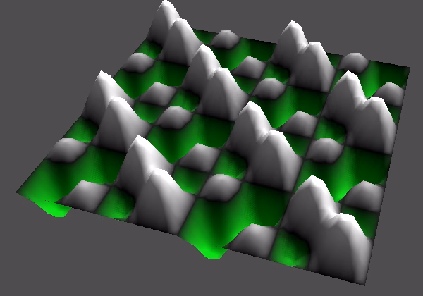
The result of adding the two samples produces a pattern with steep transitions that doesn't look much like the combination of the two patterns that we showed earlier. That's mostly because both samples are at the same strength and we showed the frequency-4 pattern at half displacement. To get the expected displacement we'll have to scale down the second sample, which we can do by multiplying it with 0.5. So we have to multiply with both its value and its derivative, so add another convenient multiply() function for that.
PatternSample add(PatternSample a, PatternSample b) {
	return PatternSample(a.v + b.v, a.d + b.d);
}

PatternSample multiply(PatternSample a, float b) {
	return PatternSample(a.v * b, a.d * b);
}
Use it to scale down the second sample.
PatternSample sample_fractal_pattern(vec2 uv) {
	return add(
			sample_pattern(base_frequency, uv),
			multiply(sample_pattern(base_frequency * 2.0, uv), 0.5)
	);
}
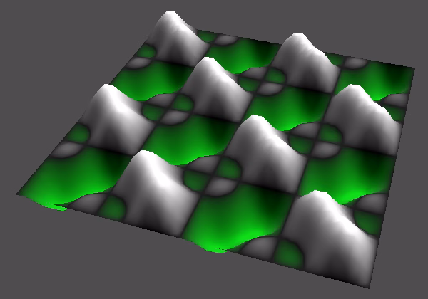
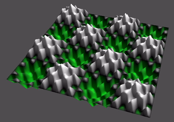
The resulting pattern might not be what you'd expect, but that's the result of sampling those two specific frequency bands and colorizing the result. Scaling the second frequency differently will produce different results. To demonstrate this let's instead multiply the base frequency with 3 for the second sample.
multiply(sample_pattern(base_frequency * 3.0, uv), 0.5) =
=
Fractal Configuration
At this point we have a very simplistic fractal with a fixed configuration. We're now going to restructure our code to make it more flexible, turning it into a loop that sums multiple samples, repeating the same relatives changes to frequency and scale for successive steps. Initially the code will still produce the same results and would likely even compile to the same instructions.
As we're summing samples we'll start with a zero sample. Let's add a convenient function to get that.
struct PatternSample {
	float v;
	vec2 d;
};

PatternSample zero_pattern_sample() {
	return PatternSample(0.0, vec2(0.0));
}
Then change sample_fractal_pattern() so its starts with a zero sample and adds the other two samples, using a sum variable to accumulate them.
PatternSample sample_fractal_pattern(vec2 uv) {
	PatternSample sum = zero_pattern_sample();
	sum = add(sum, sample_pattern(base_frequency, uv));
	sum = add(sum, multiply(sample_pattern(base_frequency * 3.0, uv), 0.5));
	return sum;
}
Let's also explicitly put the frequency that we use for the first sample in a variable, and then scale it for the second sample.
	vec2 frequency = base_frequency;
	sum = add(sum, sample_pattern(frequency, uv));
	frequency *= 3.0;
	sum = add(sum, multiply(sample_pattern(frequency, uv), 0.5));
Do the same for the scale that we apply to the sample, which starts at 1 for the first sample and is halved for the second sample. This represents the amplitude of the signal, so that's how we name it.
	vec2 frequency = base_frequency;
	float amplitude = 1.0;
	sum = add(sum, multiply(sample_pattern(frequency, uv), amplitude));
	frequency *= 3.0;
	amplitude *= 0.5;
	sum = add(sum, multiply(sample_pattern(frequency, uv), amplitude));
Then turn the code into a for loop, so we only call sample_pattern() once but loop through it twice.
	float amplitude = 1.0;
	for (int i = 0; i < 2; i++) {
		sum = add(sum, multiply(sample_pattern(frequency, uv), amplitude));
		frequency *= 3.0;
		amplitude *= 0.5;
	}
	//sum = add(sum, multiply(sample_pattern(frequency, uv), amplitude));
Octaves
Now we can add configuration variables for our fractal. Let's start with how many samples we layer on top of each other. Each sample of the pattern is known as a octave of the fractal, so we use a uniform int octaves variable for it, with a default and minimum of one octave. Of course layering many octaves will be expensive to calculate, but for demonstration purposes we set the maximum to 10. If you've designed a specific pattern you could make the amount of octaves constant, though for complex patterns the loop overhead on modern GPUs will be insignificant and unrolled loops could produce very large shaders.
uniform vec2 base_frequency = vec2(1.0);
uniform int octaves : hint_range(1, 10) = 1;
Use octaves to control how many samples get summed.
	for (int i = 0; i < octaves; i++) {
		sum = add(sum, multiply(sample_pattern(frequency, uv), amplitude));
		frequency *= 3.0;
		amplitude *= 0.5;
	}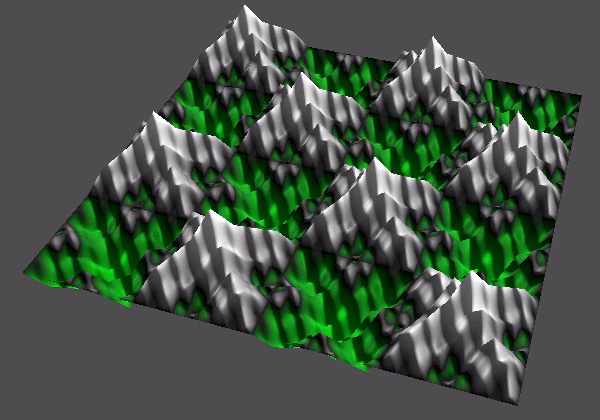
The amount of octaves affects the details of the fractal. More octaves means more details.
Persistence
The second configuration option is the factor with which we scale the frequency per octave. This controls how quickly successive octaves fade out and is known as the fractal's persistence, which goes from 0 to 1 and has a default of 0.5.
uniform int octaves : hint_range(1, 10) = 1;
uniform float persistence : hint_range(0.0, 1.0, 0.05) = 0.5;
Use persistence to scale the amplitude in the loop.
	for (int i = 0; i < octaves; i++) {
		sum = add(sum, multiply(sample_pattern(frequency, uv), amplitude));
		frequency *= 3.0;
		amplitude *= persistence;
	}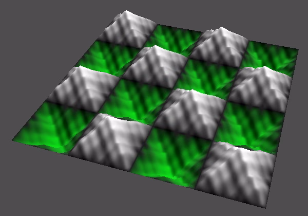
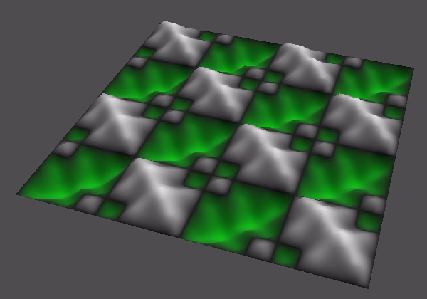
Persistence controls the strength of the details of the fractal. Low persistence produces smooth patterns, while high persistence produces rugged patterns.
Lacunarity
The third configuration option is known as the fractal's lacunarity, which is a measure of how it fills space. For our purposes it is the factor that we use to scale the frequency of successive octaves. It is usually 2 so we use that as the default. At 1 each octave is the same so that's useless, but we use that for the minimum so you see what gradually increasing lacunarity looks like. We set the maximum to 5, because high lacunarity values will quickly produce frequencies that are too high to be useful.
uniform int octaves : hint_range(1, 10) = 1;
uniform float lacunarity : hint_range(1.0, 5.0, 0.1) = 2.0;
Use lacunarity to scale the frequency in the loop.
	for (int i = 0; i < octaves; i++) {
		sum = add(sum, multiply(sample_pattern(frequency, uv), amplitude));
		frequency *= lacunarity;
		amplitude *= persistence;
	}

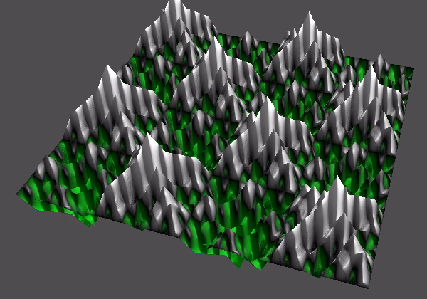
Low lacunarity makes the detail level increases slowly per octave, which produces smoother patterns, while high lacunarity makes the detail level increases quickly per octave, producing grainier patterns.
Normalized Fractal Pattern
Summing multiple samples can produce a final pattern with an amplitude greater than one, which means that it goes outside the bounds of our color gradient. We can visualize the values that are too extreme by first checking whether the value's absolute value exceeds 1 in colorize(). If so we make the color magenta.
vec3 colorize(float v) {
	if (abs(v) > 1.0) {
		return vec3(1.0, 0.0, 1.0);
	}
	if (v >= 0.0) {
		return vec3(v);
	}
	else {
		return vec3(0.0, -v, 0.0);
	}
}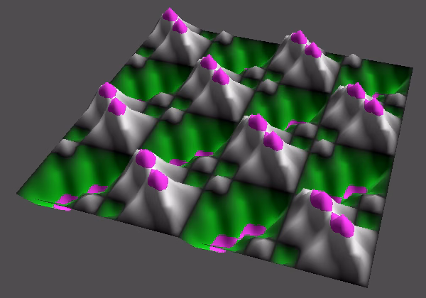
Now out-of-bounds values appear as magenta and we see that the peaks and valleys of our pattern are too extreme. Ideally our pattern stays within the expected range, so let's introduce a normalize_fractal_sample() function that scales a sample so it will stay in the −1–1 range. We start with scaling with 1 and will figure out the correct scale in a moment. Use this function to normalize the sum at the end of sample_fractal_pattern().
PatternSample normalize_fractal_sample(PatternSample s) {
	float scale = 1.0;
	return multiply(s, scale);
}

PatternSample sample_fractal_pattern(vec2 uv) {
	…
	return normalize_fractal_sample(sum);
}
Fixed Scale
Let's first consider a perfect fractal, which has an infinite amount of octaves. If persistence is 0 then that's the same as having only one octave, so we should not scale at all, which means that we should use a scale of 1.
If persistence is 1 then infinite octaves would blow up the pattern to infinity as well, so the only sensible scale would be 0.
If persistence is 0.5 then the second octave pushes the fractal's amplitude to 1.5, halfway form 1 to 2. The third octaves pushes it from 1.5 to 1.75, halfway from 1.5 to 2. So each successive octaves halves the remaining distance to 2. We have the sum of 1 + ½ + ¼ + …, which taken to infinity gives us 2. So we should divide by 2, which means the scale should be 0.5.
In general the fractal's amplitude is equal to the sum of its persistence raised raised to the power of n, with n going from 0 to infinity. Using p for persistence, this gives us the WolframAlpha function sum p^n, n = 0 to inf and we get 1/(1-p), so our scale factor is 1-p.
float scale = 1.0 - persistence;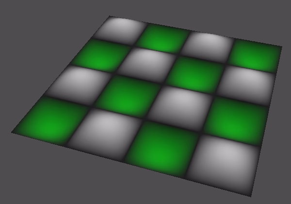
Note that we assume that all octaves can work together to reach the theoretical maximum possible amplitude. In practice this maximum would rarely be reached, or not at all, depending on the pattern. So normalizing the pattern will always make it appear weaker.
Adaptive Scale
The fixed scale factor that we use guarantees that the fractal's amplitude never exceeds 1, but it can only gets close its theoretical maximum when many octaves are summed. If we're only summing a few octaves then the result will be weak, especially when only using a single octave. An alternative approach is to use the actual amount of octaves to scale the fractal. Because this requires more work and changes the strength of the pattern based on the amount of octaves let's make it optional. Add a uniform bool adaptive_fractal_scale variable for this.
uniform float persistence : hint_range(0.0, 1.0, 0.05) = 0.5;
uniform bool adaptive_fractal_scale = false;
To find this adaptive scale we have calculate a partial sum instead of the infinite sum from before: sum p^n, n = 0 to k, which is (pk+1-1)/(p-1). Here k starts at zero, which represents the first octave, so k+1 equals the amount of octaves. If we directly use the octaves for k we can simplify to (pk-1)/(p-1). Then we can negate both the numerator and denominator and end up with (1-pk)/(1-p), which leads to the scale factor (1-p)/(1-pk).
So to make the scale factor adaptive we have to divide what we already have by 1-pk. We can perform the exponentiation via pow(), converting octaves to a float.
	float scale = 1.0 - persistence;
	if (adaptive_fractal_scale) {
		scale /= 1.0 - pow(persistence, float(octaves));
	}
	return multiply(s, scale);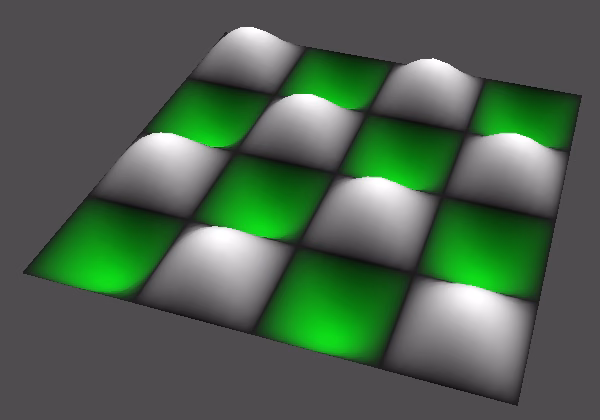

Shouldn't pow() be avoided?
Using pow() with arbitrary exponents is relatively expensive, so avoiding it is a good idea in general. We could also accumulate the scale divisor in the fractal loop, but that would make our code more complex and harder to manage. For maximum performance its calculation can be avoided entirely by using either a constant or setting it via a uniform variable. But for simplicity and flexibility we calculate it in the shader.
At this point using a persistence of 1 doesn't make sense anymore, because that will set the fixed scale to zero, while calculating the adaptive scale will lead to a division by zero, so let's limit it to 0.95.
uniform float persistence : hint_range(0.0, 0.95, 0.05) = 0.5;The next tutorial is Hashing.